Multi-Head Attention: Many Eyes on the Data

Why One Head Isn’t Enough

A single self-attention head computes one set of relevance scores across all token pairs. But language is rich: in one sentence, “bank” might need to attend to “river” for its meaning AND to “withdrew” for its syntactic role — simultaneously.

With a single head, the model must average these signals into one distribution, losing specificity. Multiple heads solve this by each specialising in a different type of relationship.

Intuition First: Why Multiple Lenses?

Think about how you understand a sentence like “The bank by the river approved the loan.”

To fully understand “bank” you need to resolve two things simultaneously:

• Its syntactic role (it is the grammatical subject)
• Its semantic disambiguation (river context → geographical bank, not financial)

A single attention head must blend these two signals into one distribution. Head A might focus on syntax while Head B focuses on nearby context — and the final linear layer W_O combines both views.

The Idea: Parallel Subspaces

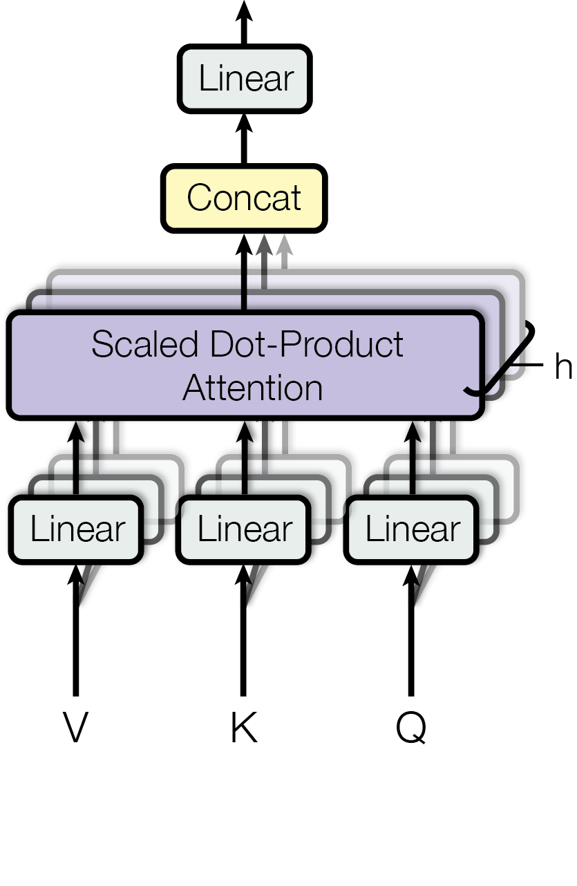
Instead of computing attention once in the full d-dimensional space, Multi-Head Attention:

1. Splits the Q, K, V matrices into h smaller pieces (each of dimension d/h).
2. Runs scaled dot-product attention independently on each piece (each piece = one “head”).
3. Concatenates the h output matrices.
4. Projects the concatenated result back to the original dimension with a final weight matrix W_O.

In Numbers

The original “Attention Is All You Need” paper uses:

• Model dimension: d_model = 512
• Number of heads: h = 8
• Head dimension: d_k = d_v = 512 / 8 = 64

So each head works in a 64-dimensional subspace — much cheaper per head, but collectively richer than a single 512-dim head.

The formula is simply:

where:

What Each Head Learns

Research on attention visualisation (e.g., BERTology papers) shows that different heads naturally specialise:

• Some heads track syntactic dependencies (subject–verb agreement).
• Some heads track co-reference (resolving “it” → “animal”).
• Some heads track positional proximity (attending mostly to adjacent tokens).
• Some heads look broadly across the whole sequence.

This specialisation emerges from training; nobody explicitly assigns these roles.

Worked Example: 2 Heads, d_model = 4

Let d_model = 4 and h = 2, so each head works in d_k = d_v = 2 dimensions.

Suppose one token has embedding x = [1, 0, 1, 0].

Head 1 uses W_Q1, W_K1, W_V1 projected onto dimensions 0–1. It might learn to track syntactic role.

Head 2 uses W_Q2, W_K2, W_V2 projected onto dimensions 2–3. It might learn to track semantic meaning.

Each head produces a 2-dimensional output. After two heads compute their results:

head₁ output: [a, b]     (syntactic view)
head₂ output: [c, d]     (semantic view)

Concat: [a, b, c, d]     (back to d_model = 4)
× W_O:  final 4-dim output

W_O mixes both views — it can learn to weight syntactic information from head₁ more heavily for certain tasks (e.g., POS tagging) or semantic information from head₂ more heavily for others (e.g., coreference).

Efficiency Note

The total compute is the same as one big attention head (d² operations), but split across h heads. GPUs parallelise this well because each head is independent. The final W_O projection is the only cross-head interaction.

References

• [1] Vaswani, A., et al. (2017). Attention Is All You Need.
• [2] https://www.sscardapane.it/alice-book/