
GIN: Graph Isomorphism Network — The Most Expressive GNN
Published:
Why Expressiveness Matters
Two different graphs that a GNN represents identically are indistinguishable by that model — it can’t learn to predict different outputs for them. The more graphs a GNN can distinguish, the more powerful it is.
A concrete failure of mean aggregation:
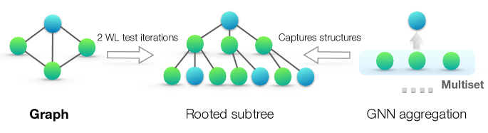
The Weisfeiler-Leman Test
The WL test is a classical algorithm for checking if two graphs are isomorphic (identical up to relabelling). It iteratively:
- Assigns a colour to each node based on its current colour + multiset of neighbour colours.
- Terminates when colours stabilise.
GNNs are essentially implementing this algorithm with learned functions. Xu et al. (2019) proved:
For a GNN to match WL, its aggregation must be an injective multiset function — a function that maps different multisets to different outputs. The key theorem:
Sum aggregation is injective for discrete features. Mean and max are not.
- Mean cannot distinguish different-sized multisets of the same elements (see figure).
- Max cannot distinguish different multiplicities of the same maximum element.
- Sum preserves both: the size of the multiset and its content.
The GIN Layer
Two components:
- ε (epsilon): a learnable (or fixed) scalar that weights the centre node’s own representation. Ensures the model treats self and neighbours differently — equivalent to a self-loop with a different weight.
- MLP: a multi-layer perceptron applied after summing. This is crucial — a single linear layer (like GCN) isn’t expressive enough to implement all injective functions. The MLP can approximate any continuous function.
Comparison
| Model | Aggregator | Update | WL power |
|---|---|---|---|
| GCN | Normalised sum | Linear + ReLU | < WL |
| GAT | Attention-weighted sum | Linear + ReLU | < WL |
| GraphSAGE | Mean | Linear + ReLU | < WL |
| GIN | Sum | MLP | = WL |
GIN is the unique architecture in this list that’s as powerful as the WL test.
GIN for Graph Classification
For graph-level tasks, GIN uses a readout that concatenates the sum-pooled representations from all layers (not just the final one):
h_G = CONCAT( SUM({h_v^k : v ∈ V}) for k=0,1,...,K )
Using representations from all layers captures both fine-grained (early layers) and coarse (late layers) structural information.
✅ Key Takeaways
- GNNs are bounded by the Weisfeiler-Leman graph isomorphism test in expressiveness.
- GIN achieves WL-equivalent expressiveness using sum aggregation + MLP update.
- Mean and max aggregation are provably less expressive — they lose information about multiset size or multiplicity.
- The ε parameter allows GIN to weight the centre node differently from its neighbours.