
GAT: Graph Attention Networks
Published:
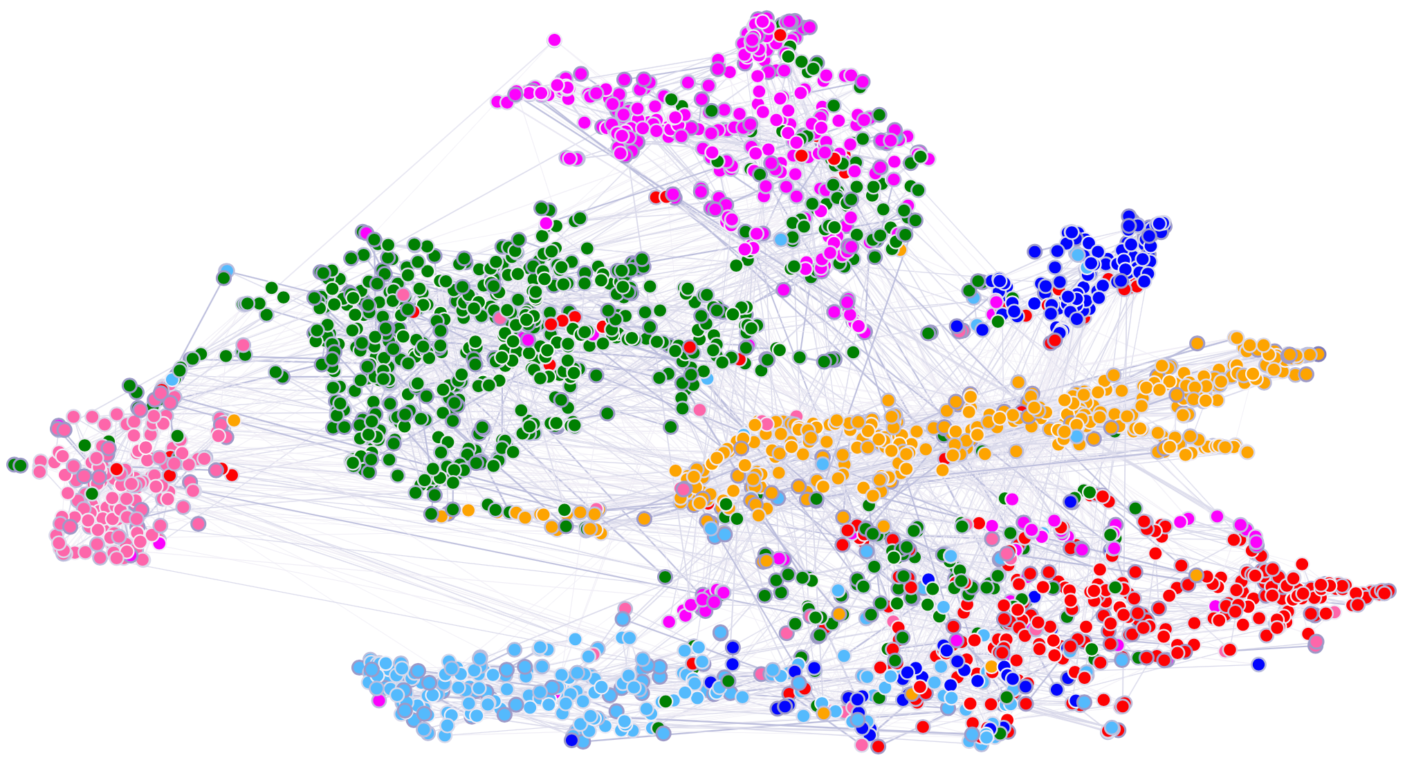
The Problem with Fixed Weights
In GCN, the aggregation weight for neighbour \(u\) contributing to node \(v\) is fixed at \(1/\sqrt{\tilde{d}_u \tilde{d}_v}\), where \(\tilde{d}_u\) is the degree of \(u\) counting its self-loop. This depends only on node degrees, the model can’t learn that some neighbours are more important than others for the task at hand.
For a citation network: when predicting paper topic, citing a paper on the exact same topic should count more than citing a survey that covers dozens of topics. GCN can’t express this.
GAT solves it by learning attention weights from features.
The Attention Mechanism
For each directed edge \(j \to i\), GAT computes an attention coefficient \(\alpha_{ij}\), how much node \(i\) attends to neighbour \(j\). Throughout, \(h_i \in \mathbb{R}^{F}\) is the input representation of node \(i\), \(W \in \mathbb{R}^{F' \times F}\) is a weight matrix shared by all nodes, and \(\mathcal{N}(i)\) is the neighbourhood of \(i\) (in the paper this includes \(i\) itself, so a node also attends to its own features).
Step 1: Linear transform. Apply the shared weight matrix \(W\) to both node features:
Step 2: Concatenate and score. Compute a raw attention score with a learned vector \(\mathbf{a} \in \mathbb{R}^{2F'}\):
Here \(\Vert\) is concatenation and the LeakyReLU uses a negative slope of \(0.2\).
Step 3: Softmax over neighbours. Normalise the scores across all neighbours of \(i\), so that they form a distribution:
Step 4: Weighted aggregate.
Note that \(\alpha_{ij} \ne \alpha_{ji}\) in general: the normalisation is per receiving node, so attention is asymmetric even on an undirected graph.
Concrete Numerical Example: Computing One Attention Coefficient
Suppose \(W = \begin{bmatrix} 1 & 0 \\ 0 & 1 \end{bmatrix}\) (the identity, for clarity), and the attention vector \(\mathbf{a} = [1, 1, 1, 1]\) (4-dimensional, matching the concatenation of two 2-dimensional vectors).
Node \(i\) has \(h_i = [1, 0]\) and neighbour \(j\) has \(h_j = [0, 1]\).
Step 1, Linear transform:
Step 2, Concatenate and score:
Step 3, Softmax over neighbours. Suppose \(i\) has one other neighbour \(k\), with raw score \(e_{ik} = 1\):
Step 4, Weighted aggregate:
Neighbour \(j\) gets roughly \(2.7\times\) the weight of \(k\).
Multi-Head GAT
Just like Multi-Head Attention in Transformers, GAT can run \(K\) independent attention heads, each with its own \(W^k\) and \(\mathbf{a}^k\) (and therefore its own coefficients \(\alpha^k_{ij}\)):
- For intermediate layers, concatenate the \(K\) head outputs, this multiplies the feature dimension by \(K\):
- For the final layer, average the \(K\) head outputs instead, which keeps the output dimension:
Each head can specialise in different types of relationships, exactly as in Transformer multi-head attention.
GAT v2 (2022)
The original GAT has a subtle expressiveness issue. Because \(\mathbf{a}\) is applied after the concatenation but before the non-linearity, the score decomposes as \(e_{ij} = \operatorname{LeakyReLU}(\mathbf{a}_1^{\top} z_i + \mathbf{a}_2^{\top} z_j)\), and the term \(\mathbf{a}_1^{\top} z_i\) is the same for every \(j\). Since LeakyReLU is monotonic, the ranking of neighbours by attention score is therefore identical for every query node \(i\), attention that is static rather than query-dependent. Brody et al. (2022) named and proved this.
GAT v2 fixes it with a small change, applying the non-linearity before the dot product with \(\mathbf{a}\):
Now the non-linearity mixes the two nodes before \(\mathbf{a}\) scores them, so the attention is dynamic: a genuine function of the pair \((i, j)\), and each node can induce its own ranking over its neighbours.
When to Use GAT over GCN?
- When neighbour importance varies and you want the model to learn which neighbours matter.
- When interpretability is important, the \(\alpha_{ij}\) values can be visualised as edge importance scores (though attention weights should be read as a hint, not a faithful explanation).
- When edge features are available (they can be concatenated into the attention score).
✅ Key Takeaways
- GAT replaces GCN's fixed degree weights with learned attention coefficients \(\alpha_{ij}\) on each edge, normalised by a softmax over \(\mathcal{N}(i)\).
- Attention is computed from both endpoints' features, adaptive to the task, not just graph topology, and is asymmetric: \(\alpha_{ij} \ne \alpha_{ji}\).
- Multi-head GAT runs \(K\) attention heads in parallel: concatenated in intermediate layers, averaged in the final one.
- GAT v2 fixes the original's static attention, a neighbour ranking shared by every query node, by applying the non-linearity before the scoring vector \(\mathbf{a}\).