
Let the Heads Talk: Beyond Diagonal Graph Attention
Published:
Authors: Riccardo Ali* (University of Cambridge), Alessio Borgi* (University of Cambridge & Sapienza University of Rome), Mario Severino* (University of Cambridge & University of Padua), Alessio Gravina (University of Pisa), Davide Bacciu (University of Pisa), Pietro Liò (University of Cambridge), Christopher Irwin* (University of Cambridge), *equal contribution
Preprint: arXiv:2610.01494, October 2026
In plain words: a multi-head attention layer is a team of specialists who each listen to the neighbours on their own private channel. Top-A lets the message travelling along each connection be re-routed between channels, so what one specialist hears from a particular neighbour can also reach a colleague, and different neighbours can be re-routed differently. If re-routing turns out to be useless, the model switches it off and is ordinary attention again. The bigger point: the “matrix on every edge” that sheaf networks are built around and the “many heads” that attention is built around are the same idea seen from two sides.
What is a sheaf actually good for?
Sheaf neural networks begin from an appealing idea. In a GCN or a GAT, a neighbour’s message is reweighted: multiplied by a scalar, from a fixed normalisation or a learned attention score, then summed. In a sheaf network the message is transformed: each edge carries a linear map, and a neighbour’s features pass through that matrix before they arrive. Since Neural Sheaf Diffusion, that richer transport has been the reason sheaves were supposed to help with heterophily and oversmoothing.
Two things have made the picture blurrier.
First, the classical construction couples several moving parts. Restriction maps send node features into an edge space, their composition induces node-to-node transport, and the sheaf Laplacian assembles everything into a diffusion. If a sheaf model wins, which part earned the win? Recent architectures increasingly skip the scaffolding and learn edge-dependent matrices directly, as in copresheaf networks and Cooperative Sheaf Neural Networks.
Second, the motivating claims are under pressure. Hernandez Caralt et al. (2026) and Fiorini et al. (2026) both question whether the gains under heterophily and oversmoothing come from the learned sheaf structure at all.
So the paper asks something more basic than “when do sheaf networks beat GNNs?”:
From sheaves to quivers: keep only the transport
The first move is to isolate the object that matters.
A quiver representation writes that operator down directly and forgets how it was built. Treat the computational graph as a quiver: vertices are nodes, and every directed interaction \(j\to i\) is an arrow. A representation assigns a vector space \(Q(i)\) to every vertex and a linear map to every arrow,
\[T_{i\leftarrow j}: Q(j)\longrightarrow Q(i), \qquad \mathbf{x}_i^{(\ell)}=\sum_{j\in\mathcal{N}(i)} T^{(\ell)}_{i\leftarrow j}\,\mathbf{x}_j^{(\ell-1)} .\]The sheaf message is the special case \(T_{i\leftarrow j}=\mathcal{F}_{i\to e}^{\top}\mathcal{F}_{j\to e}\). Everything else, the factorisation through the edge stalk and the diffusion operator, is set aside. This follows Hajij et al.’s copresheaf networks, which cast topological message passing as local maps on quiver arrows.
One difference arrives for free. A sheaf on an undirected edge couples the two directions: \(T_{j\leftarrow i}=T_{i\leftarrow j}^{\top}\), transpose reciprocity. A quiver gives \(j\to i\) and \(i\to j\) independent maps. Classical sheaf transport is the undirected special case of the object studied here.
With transport isolated, the next step is to look for it somewhere unexpected.
Multi-head attention is diagonal transport
Recall what an attention head does on a graph. Head \(h\) produces a value \(V_j^{(h)}\in\mathbb{R}^{C}\) for sender \(j\), a score for the interaction \(j\to i\), and a receiver-normalised coefficient
\[\alpha^{(h)}_{i\leftarrow j}=\frac{\exp s^{(h)}_{i\leftarrow j}}{\sum_{k\in\mathcal{N}_{\text{att}}(i)}\exp s^{(h)}_{i\leftarrow k}}, \qquad M^{(h)}_i=\sum_{j\in\mathcal{N}_{\text{att}}(i)}\alpha^{(h)}_{i\leftarrow j}V^{(h)}_j ,\]where \(\mathcal{N}_{\text{att}}(i)\) is the local neighbourhood for a GAT-style layer or every node for a graph transformer.
The usual way to read multi-head attention is “\(H\) independent attention patterns, concatenated”. The paper reads it differently: take the heads themselves as the coordinates of the local space, \(Q(i)=\mathbb{R}^{H}\), and carry each head’s \(C\)-dimensional content along in parallel. Stack a sender’s values as \(V_j\in\mathbb{R}^{H\times C}\). For the interaction \(j\to i\), the attention coefficients form a matrix,
\[D_{i\leftarrow j}=\operatorname{Diag}\!\left(\alpha^{(1)}_{i\leftarrow j},\dots,\alpha^{(H)}_{i\leftarrow j}\right)\in\mathbb{R}^{H\times H}, \qquad M^{\text{att}}_i=\sum_{j}D_{i\leftarrow j}\,V_j .\]That is a quiver representation. Every edge carries a linear map on head space, and the map is diagonal.
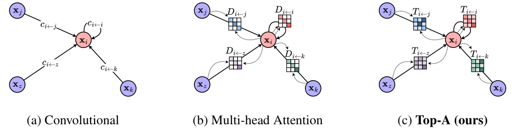
The appendix closes the loop from the other side. Call attention symmetric if \(\alpha^{(h)}_{i\leftarrow j}=\alpha^{(h)}_{j\leftarrow i}\ge 0\) for every head. Choosing restriction maps \(\mathcal{F}_{i\to e}=\mathcal{F}_{j\to e}=D_{i\leftarrow j}^{1/2}\) gives \(\mathcal{F}_{i\to e}^{\top}\mathcal{F}_{j\to e}=D_{i\leftarrow j}\) exactly (Proposition B.2). Symmetric multi-head attention is a diagonal cellular sheaf. The two literatures were describing the same object from opposite ends.
The bridge: one object, two vocabularies
That pair of propositions is the paper’s central contribution and the reason this post sits in two books of this blog. Attention and sheaf neural networks have developed in parallel for years, with separate papers, benchmarks and intuitions. Through the quiver lens they become two descriptions of the same mathematical object: a linear map attached to every directed edge, acting on a small local space.
| Attention view | Sheaf view | Unified (quiver) view | |
|---|---|---|---|
| Local space at a node | the \(H\) attention heads | the stalk \(\mathcal{F}(i)\) | \(Q(i)=\mathbb{R}^H\) |
| What crosses an edge | per-head scores \(\alpha^{(h)}_{i\leftarrow j}\) | restriction maps \(\mathcal{F}_{i\to e}^{\top}\mathcal{F}_{j\to e}\) | a linear map \(T_{i\leftarrow j}\) |
| Shape of that map | diagonal \(D_{i\leftarrow j}\) | full, symmetric across directions | full and directed |
| Data dependence | scores from \(\mathbf{x}_i,\mathbf{x}_j\) | maps predicted from \(\mathbf{x}_i,\mathbf{x}_j\) | interaction descriptor \(\xi_e\) |
| Where they meet | symmetric attention | diagonal sheaf, \(\mathcal{F}_{i\to e}=D^{1/2}_{i\leftarrow j}\) | Proposition B.2: equal |
- From sheaves to attention: the sheaf literature's central claim, that edges should transform messages rather than merely reweight them, tells attention what it is missing. Multi-head attention uses only the diagonal of the available transport; Top-A uses the rest.
- From attention to sheaves: attention's machinery, data-dependent scores, multiple heads, scalable transformer backbones, gives sheaf ideas a concrete and efficient home. The sheaf question "what is the matrix on the edge good for?" becomes a testable attention question: "when should heads exchange information along an edge?"
Readers arriving from the Transformers book can read what follows as a principled extension of multi-head attention with a sheaf-theoretic explanation; readers arriving from the Sheaf book can read it as the cleanest experiment yet on what matrix-valued transport contributes, run inside the architecture family the rest of deep learning already uses.
With the bridge in place, the next step is to cross it.
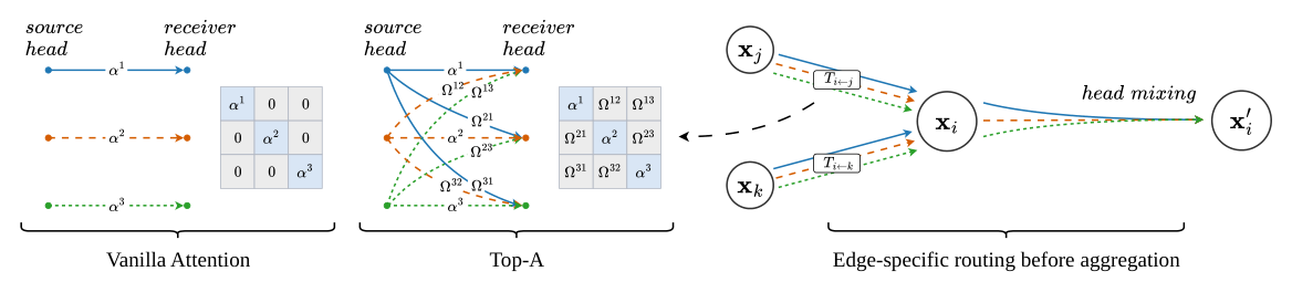
The off-diagonal entries: letting heads talk
A general head-space map \(T_{i\leftarrow j}\in\mathbb{R}^{H\times H}\) acts on the sender values as
\[\left[T_{i\leftarrow j}V_j\right]^{(r)}=\sum_{s=1}^{H}T^{rs}_{i\leftarrow j}\,V^{(s)}_j .\]An off-diagonal entry \(T^{rs}_{i\leftarrow j}\) with \(r\neq s\) lets what source head \(s\) carries flow into receiver head \(r\), on that edge. On the full representation the operator is \(T_{i\leftarrow j}\otimes I_C\): it mixes between heads and leaves the coordinates within each head alone.
Two properties make this more than a cosmetic change.
It is edge-specific. Because the map lives on a directed interaction, two senders feeding the same receiver can be routed differently, and \(j\to i\) need not mirror \(i\to j\).
It happens before aggregation. The message is transformed while it still carries the identity of the edge it came from.
The second property is where the formal result comes in, and it is why Top-A cannot be dismissed as “just another output projection”.
Topological Attention
Top-A keeps the attention coefficients and multiplies in a routing branch. For a directed interaction \(e=(j\to i)\), with \(D_e\) the usual diagonal attention operator,
Expanding for receiver head \(r\) shows what each piece does:
\[\left[M^{\text{Top-A}}_i\right]^{(r)} =\sum_{j}\alpha^{(r)}_{i\leftarrow j}\Big(\,V^{(r)}_j+\lambda\sum_{s\neq r}\Omega^{rs}_{i\leftarrow j}V^{(s)}_j\Big).\]- The first term is ordinary same-head attention, untouched: \(\operatorname{diag}(T_e)=\operatorname{diag}(D_e)\).
- The second term brings in the other heads, weighted by the routing matrix.
- Because \(D_e\) multiplies from the left, \(\alpha^{(r)}_{i\leftarrow j}\) still scales everything entering head \(r\) from that edge. Attention keeps its job of deciding how much a neighbour matters; \(\Omega_e\) decides how heads are combined inside that neighbour’s message.
- With \(\Omega_e=0\), Top-A is exactly standard multi-head attention.
Learning the routing. Each interaction gets a descriptor \(\xi_e\) built from quantities the attention layer already computes, and a small learned map turns it into routing coefficients:
\[\Omega_e=\operatorname{off}\!\big(\tanh g_\theta(\xi_e)\big), \qquad \operatorname{off}(A)=A-\operatorname{Diag}(\operatorname{diag}A).\]The \(\tanh\) bounds the coefficients and allows either sign; \(\operatorname{off}(\cdot)\) removes the diagonal so routing only ever acts between different heads. For GATv2, \(\xi_e\) is the same directed sender–receiver pre-activation the attention score uses (receiver and sender projections plus edge and graph features); for the Graph Transformer, it combines the receiver query with the edge-conditioned sender key.
One forward pass, step by step. For a receiver \(i\) with \(H\) heads:
- Compute attention scores and values as usual; for each incoming edge this gives \(D_{i\leftarrow j}\) and \(V_j\).
- From the same intermediate quantities, form the interaction descriptor \(\xi_{i\leftarrow j}\).
- Map it to an \(H\times H\) matrix, squash with \(\tanh\), zero the diagonal: \(\Omega_{i\leftarrow j}\).
- Transform each neighbour’s message individually: \(T_{i\leftarrow j}V_j=D_{i\leftarrow j}(V_j+\lambda\,\Omega_{i\leftarrow j}V_j)\).
- Only now sum over neighbours, then apply the usual head mixing and output projection.
Steps 2 to 4 are the whole addition; everything else is the backbone’s own code.
| Cost. Generating and applying a dense \(H\times H\) map per edge adds $$\mathcal{O}\big( | \mathcal{E} | \,H^2(p+C)\big)\(compute, with\)p\(the descriptor size, and\)\mathcal{O}( | \mathcal{E} | H^2)$$ memory if the maps are stored. With the usual handful of heads the overhead stays small: on MovieLens, about 7% more parameters for GATv2 (28,416 → 30,496). |
Why a projection after aggregation is not enough
The obvious objection: attention layers already end with an output projection that mixes heads. Why not let that do the cross-head work?
The answer is about order of operations, and the paper makes it exact. Stack sender values as \(\mathbf{v}_j\in\mathbb{R}^{HC}\) and write the full-size operators \(\mathbf{D}_{i\leftarrow j}=D_{i\leftarrow j}\otimes I_C\) and \(\mathbf{T}_{i\leftarrow j}=T_{i\leftarrow j}\otimes I_C\).
Note how generous the comparison is: \(A\) may be any receiver-specific linear map, far more flexible than the single shared projection a real attention layer uses. It still fails.
The two-edge example in the appendix makes the reason tangible. A receiver has two senders, both heads attend equally to both (\(D=\tfrac12 I_2\)), and the edges route differently:
\[\Omega_{i\leftarrow j_1}=\begin{pmatrix}0&\rho\\0&0\end{pmatrix}, \qquad \Omega_{i\leftarrow j_2}=\begin{pmatrix}0&0\\\rho&0\end{pmatrix}.\]Send \(\mathbf{v}=(1,0)^{\top}\) from \(j_1\) and nothing from \(j_2\), or the reverse. Standard attention produces \(\tfrac12\mathbf{v}\) both times, so anything applied afterwards must give identical outputs. Top-A produces \(\tfrac12(1,0)^{\top}\) in one case and \(\tfrac12(1,\rho)^{\top}\) in the other.
That settles what Top-A can express. Whether it helps is an empirical question, and the paper tests it on settings chosen to answer it.
Where cross-head transport earns its keep
The evaluation is built around a hypothesis rather than a leaderboard: edge-conditioned cross-head transport should help when individual interactions call for different transformations of what they carry. Each benchmark probes a different version of that, with GATv2 and a Graph Transformer (GT) as backbones and every Top-A model compared to its own baseline under an identical pipeline.
Relational reasoning on STaR
STaR is a controlled benchmark where the edge label is the computation. Each instance is a graph whose edges carry qualitative relations, spatial ones from RCC-8 (8 relations) or temporal ones from Allen’s Interval Algebra (13 relations), plus a query pair of nodes. The model must infer the relation between them by composing relations along paths and combining the partial, possibly disjunctive, evidence from several paths. Different relations demand different transformations of the propagated state: the textbook case for edge-conditioned transport.
Each domain has 57,600 training and 153,600 test instances. Models train on path length \(k\in\{2,3,4\}\) and up to \(b=3\) paths, run 15 shared-weight recurrent rounds, and are tested on depths up to \(k=15\).
| Architecture | Variant | RCC-8 ↑ | Interval Algebra ↑ |
|---|---|---|---|
| GATv2 | – | 39.79 ± 23.83 | 18.05 ± 17.94 |
| Top-A | 51.79 ± 7.14 | 52.44 ± 1.22 | |
| GT | – | 23.34 ± 17.68 | 18.03 ± 15.69 |
| Top-A | 60.24 ± 10.21 | 57.17 ± 2.54 |
Accuracy over 3 seeds. Two things stand out beyond the means. On Interval Algebra, Top-A roughly triples accuracy for both backbones. And look at the standard deviations: the baselines swing by ±16 to ±24 points between seeds, the Top-A variants by ±1 to ±10. The same relational information is available to both arms, since relation labels feed the attention scores too; what Top-A adds is the ability for each labelled edge to reroute information between heads rather than only rescale it.
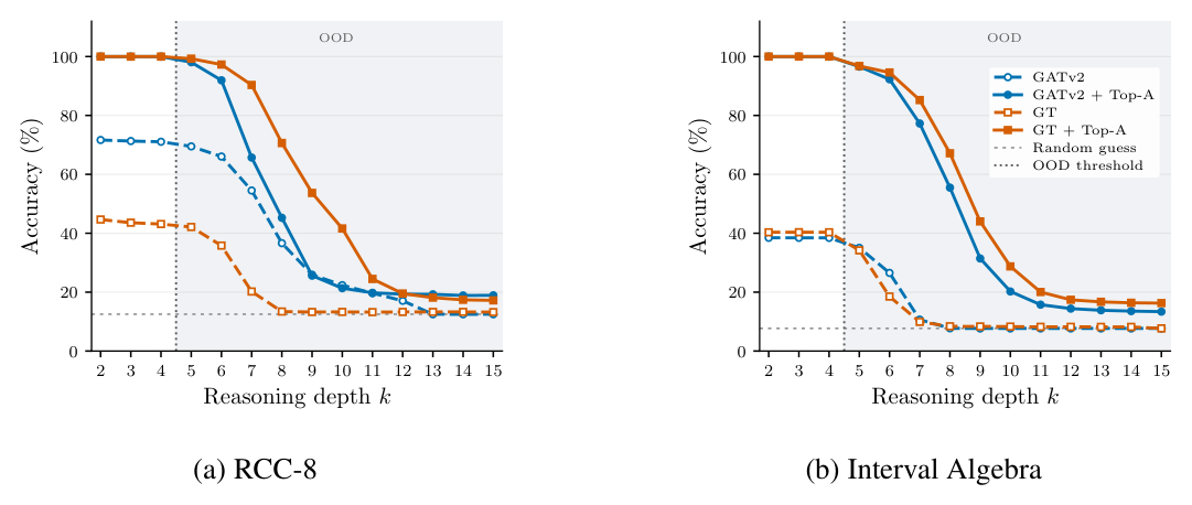
The depth curves tell the honest version of the story. Within the training range, Top-A sits near 100% where the baselines plateau between 40% and 70% (RCC-8) or around 40% (Interval Algebra). The advantage carries well past the training depths, then narrows on the longest chains, where every model drifts towards random guessing.
Heterogeneous graphs: MovieLens-100K
Next, a real heterogeneous graph: 943 users and 1,682 movies, each rating producing two directed interactions, rates (user → movie) and rated-by (movie → user). The task is binary link prediction, with type-specific encoders, relation type as an edge feature available to both attention and routing, and ten evaluation seeds disjoint from the tuning seeds.
| Model | Variant | AUROC ↑ | AUPR ↑ |
|---|---|---|---|
| GATv2 | – | 88.70 ± 0.83 | 86.48 ± 1.07 |
| Top-A | 90.46 ± 0.42 | 88.71 ± 0.51 | |
| GT | – | 81.26 ± 3.67 | 76.24 ± 5.21 |
| Top-A | 90.20 ± 0.85 | 88.38 ± 0.99 |
Around +2 points for GATv2 and +10.5 for the GT, which closes the gap between the two backbones and shrinks the GT’s seed-to-seed spread roughly fourfold.
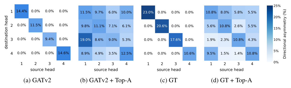
The more interesting evidence is what the routing learned. Averaging the effective transport separately over the two directions and comparing them entry by entry shows that the off-diagonal routes are used differently for rates and rated-by; vanilla attention, having no off-diagonal entries, can only differ on the diagonal.
Projecting each edge’s twelve off-diagonal routing coefficients onto two principal components and colouring by movie genre goes one step further: Drama/Mystery/Thriller, Action/Adventure/Sci-Fi and Children’s/Animation movies land in different regions, clearly for rated-by edges and more weakly for rates. Genre is never a training target, so the routing varies with node content, not only with the discrete relation type.
Algorithmic reasoning: CLRS-30
CLRS covers 30 textbook algorithms across eight families, trained at size \(n=16\) and tested out of distribution at \(n=64\). The point here is not a uniform gain; it is to see which computations want cross-head routing. All four variants are tuned separately with the same budget, then evaluated on 20 seeds.
| Family | Tasks | GATv2 | + Top-A | Δ | GT | + Top-A | Δ |
|---|---|---|---|---|---|---|---|
| Sorting | 4 | 25.18 | 54.42 | +29.24 | 23.81 | 54.17 | +30.36 |
| Searching | 3 | 42.31 | 54.72 | +12.41 | 31.92 | 56.24 | +24.32 |
| Divide and conquer | 1 | 58.10 | 63.61 | +5.51 | 57.19 | 62.91 | +5.72 |
| Greedy | 2 | 74.22 | 73.92 | −0.30 | 74.98 | 73.94 | −1.03 |
| Dynamic programming | 3 | 73.54 | 73.71 | +0.17 | 76.34 | 70.02 | −6.32 |
| Graphs | 12 | 60.68 | 61.86 | +1.18 | 54.51 | 60.51 | +5.99 |
| Strings | 2 | 1.39 | 1.54 | +0.15 | 1.40 | 1.92 | +0.53 |
| Geometry | 3 | 70.26 | 72.63 | +2.36 | 70.04 | 71.59 | +1.55 |
| Overall | 30 | 53.22 | 59.26 | +6.04 | 49.81 | 58.36 | +8.56 |
Official CLRS score, %, mean over 20 seeds (standard deviations in the paper).
The pattern is the result. Sorting and searching jump by roughly 30 and 12 to 24 points; individual tasks move far more: binary search from 5.6% to 79.9% with the GT, insertion sort from 28.5% to 84.5% with GATv2, quicksort and bubble sort each by more than 37 points. The GT also gains strongly on shortest paths: Dijkstra +21.5, Bellman–Ford +13.8, Floyd–Warshall +12.2. Greedy algorithms and dynamic programming barely move or get worse, and some tasks regress outright: heapsort drops for both backbones, and optimal BST loses 15.9 points with the GT. The task-averaged score still improves on all 20 seeds for both architectures.
Sorting and searching are procedures where an element’s role changes depending on whom it is being compared with. Routing information between head subspaces per comparison appears to match that structure; procedures built on monotone, local accumulation do not seem to need it.
The contrast setting: heterophily
Heterophily was the original sales pitch for matrix-valued sheaf transport: when neighbours differ, transform their messages rather than merely reweight them. If that pitch were the whole story, Top-A should shine on the standard heterophilic benchmarks. It does not.
For readers of the sheaf book, the same table carries a second message: the sheaf baselines that do well there, CSNN and BuNN, lead on roman-empire, minesweeper, tolokers and questions, while O(d)-NSD trails the attention backbones. Whatever those models gain on heterophilic graphs, it is not the cross-head routing isolated here.
This negative result is deliberate, and it sharpens the positive ones. The benefit appears where individual interactions demand different transformations: labelled relations in STaR, directed typed relations in MovieLens, comparison-dependent roles in sorting. A graph whose neighbours merely tend to have different labels does not, by itself, demand that.
Where this sits in the sheaf story
Three threads of this book meet here.
What sheaf transport is for. The recurring lesson in this literature, from identity sheaves being competitive in Neural Sheaf Diffusion to the recent doubts about learned sheaves under heterophily, is that unrestricted matrices are not automatically useful. Top-A answers at the level of a single primitive: matrix-valued transport buys edge-conditioned communication between coordinates of the local space, before aggregation, and Theorem 4.1 says exactly why that is not reducible to anything applied afterwards.
Attention and sheaves on the same axis. Sheaf Attention Networks put attention on top of sheaf transport, GAT with matrices instead of scalars. Copresheaf attention puts a matrix within each head, acting on the \(C\) value channels head by head, a block-diagonal operator. Top-A puts the matrix between heads, on the \(H\) factor of \(\mathbb{R}^H\otimes\mathbb{R}^C\), and shows that standard attention is the diagonal of that family. It is also distinct from Talking-Heads attention and DCMHA, which mix heads at the level of attention scores and weights; Top-A moves the value content itself from one head to another.
Directed transport as the default. Like CSNN and ESNN, Top-A treats \(j\to i\) and \(i\to j\) as separate maps, with classical sheaf transport as the transpose-reciprocal special case. The MovieLens asymmetry maps are a direct picture of why that freedom matters.
None of which settles everything.
- Gains are strongly task dependent: greedy and dynamic-programming algorithms see little benefit, and individual tasks such as heapsort and optimal BST regress.
- On heterophilic node classification the routing gives no consistent improvement.
- The STaR advantage narrows on the longest reasoning chains, and those results rest on three seeds.
- Each edge pays for a dense \(H\times H\) map, which scales quadratically in the number of heads.
- Code is promised upon acceptance.
✅ Key Takeaways
- A bridge between attention and sheaf neural networks. Both are linear maps on directed edges acting on a small local space. Treating heads as that space, multi-head attention is diagonal head-space transport (Proposition 3.1): head \(r\) only reaches head \(r\). Symmetric attention is exactly a diagonal cellular sheaf (Proposition B.2).
- Quiver representations isolate the one thing sheaf networks add, the linear map on each directed edge, from restriction-map factorisation and Laplacian diffusion, and drop the transpose-reciprocity that ties the two directions of an undirected sheaf edge together.
- Top-A: \(T_e=D_e(I_H+\lambda\Omega_e)\) with zero-diagonal, \(\tanh\)-bounded, edge-conditioned routing \(\Omega_e\). Same-head attention is preserved, \(\Omega_e=0\) recovers vanilla attention, and zero initialisation makes the two models identical when training starts.
- Theorem 4.1: a post-aggregation linear map can replace the routing only if it reproduces every incoming edge's transport with one shared factor. Aggregation erases message identity, so in general it cannot.
- Results: STaR accuracy up to 60.2% from 23.3% (GT, RCC-8) and roughly tripled on Interval Algebra; MovieLens AUROC +1.8 (GATv2) and +8.9 (GT); CLRS-30 +6.04 and +8.56 points overall, with sorting +29 to +30 and searching +12 to +24.
- Heterophily alone gives no systematic benefit: cross-head transport pays off when individual interactions require different transformations, not merely when neighbours differ.
References
- Ali, R.*, Borgi, A.*, Severino, M.*, Gravina, A., Bacciu, D., Liò, P., & Irwin, C.* (2026). Let the Heads Talk: Beyond Diagonal Graph Attention. arXiv:2610.01494.
- Hansen, J., & Gebhart, T. (2020). Sheaf Neural Networks. arXiv:2012.06333.
- Bodnar, C., Di Giovanni, F., Chamberlain, B. P., Liò, P., & Bronstein, M. M. (2022). Neural Sheaf Diffusion: A Topological Perspective on Heterophily and Oversmoothing in GNNs. NeurIPS 2022.
- Hansen, J., & Ghrist, R. (2019). Toward a Spectral Theory of Cellular Sheaves. Journal of Applied and Computational Topology, 3, 315–358.
- Hajij, M., et al. (2025). Copresheaf Topological Neural Networks: A Generalized Deep Learning Framework. NeurIPS 2025.
- Ribeiro, A., Tenório, A. L., Belieni, J., Souza, A. H., & Mesquita, D. (2026). Cooperative Sheaf Neural Networks. ICLR 2026.
- Hernandez Caralt, F., Gonzàlez i Català, M., Bazaga, A., & Liò, P. (2026). On the Necessity of Learnable Sheaf Laplacians. arXiv:2603.05395.
- Fiorini, S., Coppola, E., & Liò, P. (2026). Benchmarking Sheaf Neural Networks for Inductive Tasks. arXiv:2608.02558.
- Gabriel, P. (1972). Unzerlegbare Darstellungen I. Manuscripta Mathematica, 6(1), 71–103.
- Derksen, H., & Weyman, J. (2017). An Introduction to Quiver Representations. Graduate Studies in Mathematics 184, AMS.
- Veličković, P., Cucurull, G., Casanova, A., Romero, A., Liò, P., & Bengio, Y. (2018). Graph Attention Networks. ICLR 2018.
- Brody, S., Alon, U., & Yahav, E. (2022). How Attentive are Graph Attention Networks? ICLR 2022 (GATv2).
- Shi, Y., Huang, Z., Feng, S., Zhong, H., Wang, W., & Sun, Y. (2021). Masked Label Prediction: Unified Message Passing Model for Semi-Supervised Classification. IJCAI 2021 (Graph Transformer backbone).
- Shazeer, N., Lan, Z., Cheng, Y., Ding, N., & Hou, L. (2020). Talking-Heads Attention. arXiv:2003.02436.
- Xiao, D., Meng, Q., Li, S., & Yuan, X. (2024). Improving Transformers with Dynamically Composable Multi-Head Attention. ICML 2024 (DCMHA).
- Khalid, I., & Schockaert, S. (2025). Systematic Relational Reasoning with Epistemic Graph Neural Networks. ICLR 2025 (STaR).
- Veličković, P., et al. (2022). The CLRS Algorithmic Reasoning Benchmark. ICML 2022.
- Harper, F. M., & Konstan, J. A. (2015). The MovieLens Datasets: History and Context. ACM Transactions on Interactive Intelligent Systems, 5(4).
- Platonov, O., Kuznedelev, D., Diskin, M., Babenko, A., & Prokhorenkova, L. (2023). A Critical Look at the Evaluation of GNNs under Heterophily: Are We Really Making Progress? ICLR 2023.
- Barbero, F., Bodnar, C., Sáez de Ocáriz Borde, H., & Liò, P. (2022). Sheaf Attention Networks. NeurIPS 2022 Workshop on Symmetry and Geometry in Neural Representations.