
Graph Transformers: Bringing Attention to Graphs
Published:
The Limits of Local Message Passing
Standard GNNs (GCN, GAT, GIN, GraphSAGE) aggregate information only from direct neighbours. To reach a node k hops away, you need k layers. Problems:
- Long-range dependencies: for diameter-10 graphs, you need 10 layers, causing over-smoothing
- Over-squashing: information from exponentially many nodes must be compressed through bottleneck edges (see the Over-squashing post)
- Structural rigidity: the message-passing graph IS the computation graph
The solution: full attention, every node attends to every other.
Graph Transformer Architecture
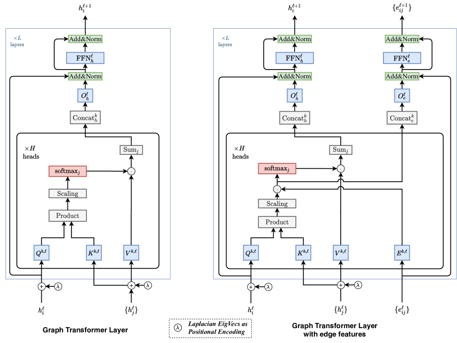
A Graph Transformer layer is essentially a standard Transformer self-attention layer, but applied to graph nodes:
Here \(b_{ij}\) is an optional attention bias encoding the graph structure between nodes \(i\) and \(j\).
Without \(b_{ij}\) and without positional encodings, the layer is permutation-invariant over the node set: it computes exactly the same thing whether the nodes form a path or a clique. The graph is simply absent from the computation. With \(b_{ij}\): graph structure guides attention (edge presence, distance, structural similarity).
The Key Challenge: Positional Encodings for Graphs
Sequences have a natural positional order (position 1, 2, 3, …). Graphs do not, there is no canonical node ordering. Without positional information, nodes with identical features but different structural roles are indistinguishable.
Graph Transformers use graph-based positional encodings (covered in depth in the Graph PE section):
- Laplacian eigenvectors: the \(k\) eigenvectors of \(L\) (or \(L_{\mathrm{sym}}\)) with the smallest non-zero eigenvalues, i.e. \(u_2, \dots, u_{k+1}\)
- Random walk PEs: the diagonal landing probabilities \(P^k[v,v]\) of a \(k\)-step walk returning to \(v\)
- Shortest path distances: encoded as learned scalar biases on attention scores
Graphormer (2021)
Graphormer (Ying et al., Microsoft) injects three structural signals:
- Centrality encoding: degree embeddings added to the node features before the QKV projection
- Spatial encoding: \(b_{ij} = \varphi\big(\mathrm{dist}(i,j)\big)\), a learned scalar per distance value, added to the attention logits
- Edge encoding: edge features along the shortest path \(i \to j\), aggregated into a second scalar bias \(c_{ij}\)
Note that the centrality term enters through the input embedding, so it is projected by \(W_Q\) and \(W_K\) along with the features, it is not added to \(q_i\) and \(k_j\) after the projection. Graphormer won the KDD Cup 2021 OGB-LSC quantum-property track (PCQM4M-LSC), and the architecture became the reference point for graph Transformers on molecules.
SAN (Spectral Attention Network)
SAN (Kreuzer et al., 2021) computes its positional encoding by running a small Transformer over the pairs \((\lambda_i, u_i(v))\), so the PE is a learned function of the spectrum rather than the raw eigenvectors. It then attends over all node pairs, but with two separate sets of query/key projections, one used when \((i,j)\) is an edge, another when it is not, with a hyperparameter \(\gamma\) balancing the two:
The point is that the model can treat “connected” and “not connected” as genuinely different relations rather than folding both into one score.
GPS (General, Powerful, Scalable Graph Transformer)
GPS (Rampášek et al., 2022) combines:
- Local message passing (GCN/GAT/GIN): captures local structural patterns efficiently
- Global self-attention (Transformer): captures long-range dependencies
GPS layer:
  h_local  ← local MPNN(h, A)    # O(|E| · d)
  h_global ← self-attention(h)   # O(N² · d)
  h_out    ← LN(h + h_local + h_global) + FFN
GPS reported strong results on the Long-Range Graph Benchmark (LRGB), a suite designed to require long-range dependency learning. Worth knowing: later work re-examined LRGB and found that carefully tuned plain MPNN baselines close much of the reported gap, so the benchmark separates architectures less cleanly than it first appeared. The hybrid design is still a sensible default; the evidence for how much the global branch buys you is weaker than headline numbers suggest.
Complexity: The \(O(N^2)\) Challenge
Full attention on a graph of \(N\) nodes costs \(O(N^2 d)\) time and \(O(N^2)\) memory, the same as self-attention in sequence Transformers, and independent of \(\lvert E\rvert\). If the model also uses a pairwise bias such as shortest-path distance, that bias matrix is itself \(O(N^2)\) to store.
For small graphs (molecules with \(N < 100\)): no problem. For large graphs (social networks with \(N > 100{,}000\)): prohibitive.
Solutions:
- Sparse or \(k\)-nearest-neighbour attention: each node attends only to a restricted candidate set
- Linear-attention / low-rank approximations: replace the softmax kernel so cost becomes linear in \(N\)
- Cluster-based: full attention within clusters, then attention between cluster summaries
- Hybrid (GPS-style): keep the sparse MPNN branch and use a cheaper global branch
Summary
| Property | Local MPNN (GCN, GAT) | Graph Transformer |
|---|---|---|
| Receptive field | \(K\)-hop (\(K\) = number of layers) | All nodes, in one layer |
| Long-range dependencies | Needs depth, which risks over-smoothing | Handled directly |
| Complexity | \(O(K \lvert E\rvert d)\) | \(O(N^2 d)\) |
| Graph structure encoding | Adjacency (message passing) | Positional encodings + attention biases |
| Suitable graph size | Any (with neighbour sampling) | Small–medium, or with an approximation |
| Over-squashing | Yes, bottleneck edges compress exponentially many paths | Removed as a topological bottleneck; finite attention capacity still limits how much can be routed |
Graph Transformers trade \(O(N^2)\) computation for the ability to connect any pair of nodes directly. On small graphs (molecules, proteins) this is a good trade. On large graphs, hybrid designs that keep a sparse local branch alongside an approximate global one are the practical frontier.
References
- Dwivedi, V. P., & Bresson, X. (2021). A Generalization of Transformers to Graphs. arXiv preprint.
- Kreuzer, D., Beaini, D., Hamilton, W. L., Létourneau, V., & Tossou, P. (2021). Rethinking Graph Transformers with Spectral Attention. NeurIPS 2021.
- Rampasek, L., Galkin, M., Dwivedi, V. P., Lim, A. T., Wolf, G., & Beaini, D. (2022). Recipe for a General, Powerful, Scalable Graph Transformer. NeurIPS 2022 (GPS).
- Vaswani, A., Shazeer, N., Parmar, N., et al. (2017). Attention Is All You Need. NeurIPS 2017.