
Equivariant Sheaf Neural Networks: Learning Geometric Transport on Graphs
Published:
Authors: Alessio Borgi* (University of Cambridge & Sapienza University of Rome), Mario Severino* (University of Cambridge & University of Padua), Fabrizio Silvestri (Sapienza University of Rome), Pietro Liò (University of Cambridge), *equal contribution
Preprint: arXiv:2608.28853, August 2026
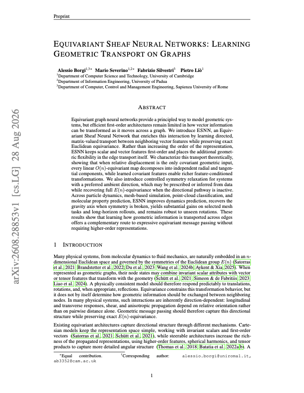
In plain words: when two connected points in a physical system talk to each other, ESNN lets the edge apply a small learned transformation to the vectors being sent, stretch along the connection, stretch differently across it, or rotate, instead of just scaling them by a number. A theorem shows this is exactly as much freedom as the symmetry laws allow, and one learnable dial, starting at zero, lets the network notice a special direction such as gravity when the data shows one.
Two literatures, one missing bridge
Geometric graph learning has spent five years perfecting two ideas that have barely spoken to each other.
On one side, equivariant GNNs. EGNN, PaiNN, GVP and their descendants carry invariant scalars and first-order Cartesian vectors, plain arrows, no higher tensors, and guarantee that if you rotate the input system, the output rotates with it. The guarantee is exact and the models are cheap, no spherical harmonics, no Clebsch–Gordan contractions. But look at what actually crosses an edge. In EGNN, the geometric content of a message is \(\phi(\lVert \mathbf{r}_{ij}\rVert)\,\mathbf{r}_{ij}\), an invariant scalar times the displacement. A neighbour’s vector features arrive isotropically scaled at best. Longitudinal and transverse responses, shear, anisotropic propagation, the direction-dependent interactions that dominate real physics, are exactly what a scalar coefficient cannot express. The steerable family (TFN, SE(3)-Transformers, MACE, EquiformerV2) buys that anisotropy by raising the representation order, features that are higher tensors, not arrows, and pays for it in tensor-product machinery.
On the other side, sheaf neural networks. Since Hansen & Gebhart’s first sheaf network and Neural Sheaf Diffusion, the sheaf literature has insisted that the interesting object on an edge is not a scalar weight but a linear map between local feature spaces. That is precisely the machinery the equivariant world is missing, matrix-valued, edge-dependent, learned transport. But every sheaf network to date treats its stalks, those local feature spaces, as abstract: nothing in a generic restriction map knows that the vectors it moves are arrows in physical space. Rotate the input point cloud and a learned restriction map does not transform accordingly. Matrix transport, no symmetry.
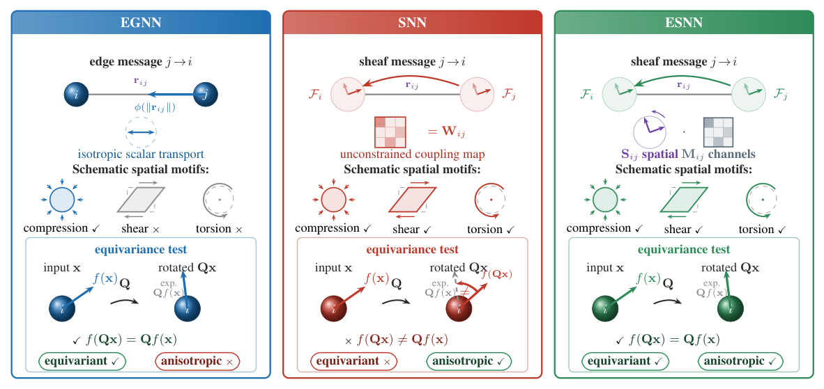
The answer turns out to be a small, fully characterised family, and that characterisation is the paper’s theoretical core.
Stop factoring through the edge
Building that bridge starts on the sheaf side, with what happens to a feature as it crosses an edge.
In classical sheaf diffusion, the contribution of node \(j\) to node \(i\) across \(e=\{i,j\}\) is, up to the Laplacian’s minus sign, the composition
, push \(j\)’s feature into the edge space, pull it back down into \(i\)’s. Every node-to-node coupling in NSD, Conn-NSD, Sheaf Attention Networks and their variants has this factored form.
ESNN’s structural move is to stop factoring. Rather than learning two incidence maps and composing them through an edge stalk, it parameterises the directed node-to-node transport itself:
The stalk now has physical structure. Each node carries \(\mathbf{h}_i=(\mathbf{s}_i,\mathbf{V}_i)\), invariant scalar channels \(\mathbf{s}_i\in\mathbb{R}^{c_s}\) and covariant vector channels \(\mathbf{V}_i\in\mathbb{R}^{n\times c_v}\), so the vector stalk is \(\mathcal{F}_{\mathrm{vec}}(i)=\mathbb{R}^n\otimes\mathbb{R}^{c_v}\). Under a rigid motion \(\mathbf{x}_i\mapsto Q\mathbf{x}_i+\mathbf{t}\), scalars stay put and vectors rotate: \(\mathbf{V}_i\mapsto Q\mathbf{V}_i\). Any legitimate transport has to commute with that action, and this single requirement is what generic sheaf parameterisations violate.
Spatial rotates, channel mixes
The vector stalk \(\mathbb{R}^n\otimes\mathbb{R}^{c_v}\) has two axes with entirely different symmetry behaviour: the spatial axis \(\mathbb{R}^n\), on which \(O(n)\) acts, and the channel axis \(\mathbb{R}^{c_v}\), on which it acts trivially. Write \(\mathrm{End}(U)\) for all linear maps \(U\to U\): since \(\mathrm{End}(\mathbb{R}^n\otimes\mathbb{R}^{c_v})\cong\mathrm{End}(\mathbb{R}^n)\otimes\mathrm{End}(\mathbb{R}^{c_v})\), every linear map on the stalk is a finite sum of separable left–right actions, one matrix multiplying each axis. ESNN’s transport is exactly that sum, with one transformation law imposed per axis:
The spatial operator \(\mathbf{S}^{(k)}_{ij}\in\mathbb{R}^{n\times n}\) multiplies from the left and must transform by conjugation when the edge’s geometric context \(\mathcal{C}_{ij}\) (displacement, endpoint vector features) is rotated, rotating the world does not change what the operator does, only the coordinates it is written in. The channel operator \(\mathbf{M}^{(k)}_{ij}\in\mathbb{R}^{c_v\times c_v}\) multiplies from the right and must be built from invariants only: the channel axis carries no geometry, so nothing there is allowed to notice the rotation at all. Proposition 3.2 verifies that these two conditions alone make the whole sum equivariant: \(\mathcal{T}'_{i\leftarrow j}(Q\mathbf{V}_j)=Q\,\mathcal{T}_{i\leftarrow j}(\mathbf{V}_j)\). Concretely, for \(n=3\), \(c_v=8\): \(\mathbf{V}_j\) is a \(3\times 8\) stack of eight arrows, each \(\mathbf{S}^{(k)}_{ij}\) a \(3\times 3\) spatial map on its rows, each \(\mathbf{M}^{(k)}_{ij}\) an \(8\times 8\) mixer on its columns.
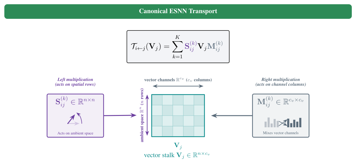
Two clarifications, then the taxonomy. The transport is linear in what it moves and nonlinear in what it reads: for a fixed edge context it acts linearly on \(\mathbf{V}_j\), while \(\mathbf{S}\) and \(\mathbf{M}\) come from networks watching the local geometry. The map adapts edge by edge, and Proposition 3.2 keeps every instance equivariant. And it is directed, \(\mathcal{T}_{i\leftarrow j}\) owes nothing to \(\mathcal{T}_{j\leftarrow i}\), a point we return to below.
Four ways to move a vector across an edge
Each choice of spatial operator instantiates a transport family.
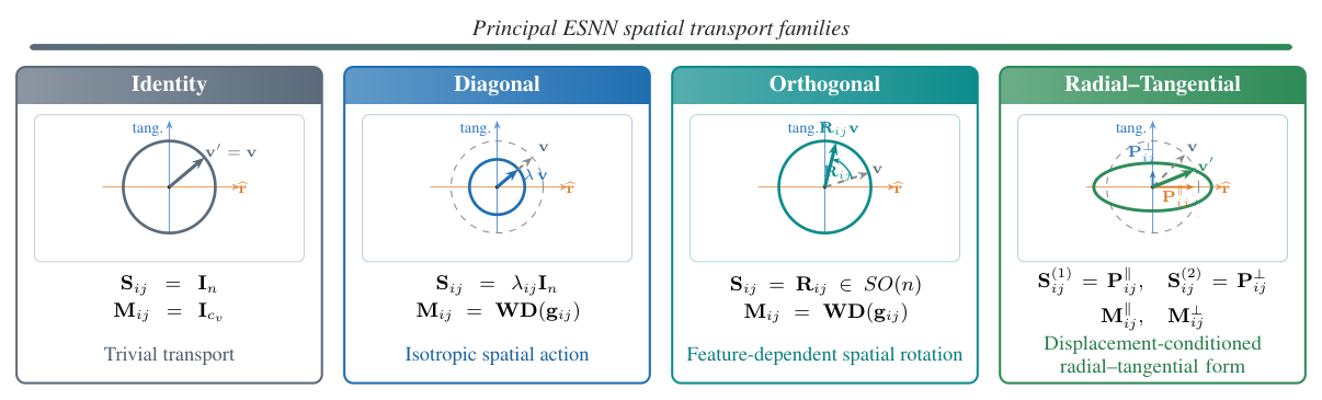
Identity. \(\mathbf{S}_{ij}=\mathbf{I}_n\), \(\mathbf{M}_{ij}=\mathbf{I}_{c_v}\): neighbours’ vectors are aggregated in the common frame untouched. This is the trivial-sheaf limit, and a useful control, any gain beyond it is attributable to learned transport rather than to the surrounding architecture.
Diagonal. \(\mathbf{S}_{ij}=\lambda_{ij}\mathbf{I}_n\) with \(\lambda_{ij}\) predicted from invariant edge features:
Edge-adaptive, but spatially isotropic, the closest ESNN analogue of what EGNN-style messages already do, plus channel mixing.
Orthogonal. The first genuinely non-trivial spatial action, and the most sheaf-flavoured one: a feature-conditioned rotation. The idea: the cross-feature matrix \(\mathbf{C}_{ij}=\mathbf{V}_j\mathbf{V}_i^{\top}\in\mathbb{R}^{n\times n}\) correlates \(j\)’s arrows with \(i\)’s, so its skew part measures the net twist between the two nodes’ feature frames. Exponentiating a learned fraction of that twist gives a rotation that can turn a neighbour’s message towards the receiver’s frame before aggregation. Concretely: Frobenius-normalise, \(\widetilde{\mathbf{C}}_{ij}=\mathbf{C}_{ij}/(\lVert\mathbf{C}_{ij}\rVert_F+\varepsilon)\), take the skew part \(\boldsymbol{\Omega}_{ij}=\widetilde{\mathbf{C}}_{ij}-\widetilde{\mathbf{C}}_{ij}^{\top}\in\mathfrak{so}(n)\), and exponentiate with an invariant learned coefficient:
Under a global rotation both the generator and its exponential transform by conjugation, \(\mathbf{R}_{ij}\mapsto Q\mathbf{R}_{ij}Q^{\top}\) for the exponential, so equivariance holds (Lemma 4.1). (“Orthogonal” names the spatial factor only: the full transport still mixes and rescales channels.) Readers of the connection-Laplacian post in the GNN book will recognise the shape: an \(SO(n)\) map per edge is parallel transport, geometry’s rule for carrying a vector along a path without extra twist. The difference is that Conn-NSD computes its orthogonal maps once from a manifold assumption, while ESNN derives them from the current features, end to end, under an ambient rather than local gauge symmetry.
Radial–Tangential. The family the theory singles out. The displacement \(\mathbf{r}_{ij}=\mathbf{x}_i-\mathbf{x}_j\) splits space into the line along the edge and its orthogonal complement:
Longitudinal and transverse components of a message get independent channel transformations. Picture a ball-and-spring network: the part of a neighbour’s motion along the spring stretches or compresses it, while the part across the spring bends it sideways, two physically different stiffnesses. EGNN’s scalar coefficient is forced to scale both identically; here each gets its own learned channel map, \(\mathbf{M}^{\parallel}_{ij}\) for the push along the bond, \(\mathbf{M}^{\perp}_{ij}\) for the shear across it. That is the anisotropy physics wants, obtained without leaving first-order features. (Self-loops, where \(\mathbf{r}_{ii}=\mathbf{0}\) defines no direction, are carried by an explicit identity self-loop in the diffusion operator instead.) And it is cheap: the projectors are never materialised, since \(\mathbf{P}^{\parallel}_{ij}\mathbf{V}_j=\widehat{\mathbf{r}}_{ij}(\widehat{\mathbf{r}}_{ij}^{\top}\mathbf{V}_j)\) costs \(\mathcal{O}(nc_v)\), keeping the layer linear in the spatial dimension.
The completeness theorem: radial–tangential is all there is
Here is the result that turns a design menu into a classification.
The proof is a stabiliser argument worth internalising, because it explains why only two projectors appear. Fix \(\mathbf{r}\neq\mathbf{0}\) and look at the subgroup that preserves it, \(H_{\mathbf{r}}=\{Q: Q\mathbf{r}=\mathbf{r}\}\cong O(n-1)\). Equivariance for these \(Q\) says the transport must commute with the stabiliser’s action. But under \(H_{\mathbf{r}}\), space decomposes as \(\mathbb{R}^n=\mathrm{span}\{\widehat{\mathbf{r}}\}\oplus\widehat{\mathbf{r}}^{\perp}\), the radial line carrying the trivial representation, the tangent space carrying the standard representation of \(O(n-1)\). The two are inequivalent, so a commuting operator cannot mix them (Schur), and on the tangent block the spatial part must be a multiple of the identity. In 3D the picture is a spin about the edge axis: it fixes the along-edge line, churns the across-edge plane, and nothing that commutes with every such spin can couple the two. What survives is \(\big(\mathbf{P}^{\parallel}\otimes\mathrm{End}(\mathbb{R}^{c_v})\big)\oplus\big(\mathbf{P}^{\perp}\otimes\mathrm{End}(\mathbb{R}^{c_v})\big)\): free channel maps on each geometric block, nothing else. Full \(O(n)\)-equivariance then forces the channel maps to depend on \(\mathbf{r}\) only through invariants like \(\lVert\mathbf{r}\rVert\).
Beyond the classified regime, ESNN offers a Unified Transport: choose any subset \(\mathcal{K}\subseteq\{\mathrm{id},\parallel,\perp,\mathrm{skew}\}\) of spatial operators and sum them as in the general definition, the four named families are its single-operator special cases. The skew member \(\widehat{\boldsymbol{\Omega}}{}^{V}_{ij}\) is the Frobenius-normalised skew matrix built from \(\mathbf{V}_j\mathbf{V}_i^{\top}-\mathbf{V}_i\mathbf{V}_j^{\top}\), used directly as a spatial operator. It is feature-conditioned and covariant: deliberately outside Theorem 4.3’s displacement-only conditioning, yet still inside Proposition 3.2’s equivariance.
Back inside the classified regime, the theorem has a practical reading. EGNN-style messages condition on displacement alone, so radial–tangential transport is not a rival design you might benchmark against them, it is the completion of the class they already live in. When displacement is all the edge sees, radial–tangential is all the linear transport there is.
The layer: five stages, one audit
The transports slot into a complete message-passing layer. One rule runs through all five stages: everything that decides is invariant; everything that moves is covariant.
1. Invariant edge context. For each directed non-self interaction, everything invariant the edge can know:
Read the bracket left to right: both endpoints’ scalars; per-channel norms \(\mathbf{n}(\cdot)\) of their vector features; a radial embedding \(\phi_r\) of the distance; per-channel inner products between the endpoints’ vectors; each endpoint’s vectors projected onto the edge direction; and any supplied invariant edge attributes. Every gate, coefficient and attention weight in the layer is predicted from this summary, so nothing that decides can endanger equivariance.
2. Transport and scalar messaging. Vector messages \(\mathbf{m}^{V}_{i\leftarrow j}=\mathcal{T}_{i\leftarrow j}(\mathbf{V}_j)\); scalar messages through a separate invariant pathway \(\mathbf{m}^{s}_{i\leftarrow j}=\mathbf{s}_j+\phi_s(\mathbf{z}^{s}_{ij})\).
3. Normalised transport diffusion. Messages aggregate under symmetrised-degree normalisation \(\nu_{ij}=\omega_{ij}/\sqrt{(\bar d_i+1)(\bar d_j+1)}\), where \(\omega_{ij}\ge 0\) is an optional invariant edge weight (unit in the unweighted case) and \(\bar d_i=\tfrac{1}{2}\big(\sum_j\omega_{ij}+\sum_j\omega_{ji}\big)\) the symmetrised degree, with an explicit identity self-loop \(\nu_{ii}=1/(\bar d_i+1)\). In words: GCN’s \(\tilde D^{-1/2}\tilde A\tilde D^{-1/2}\) normalisation, self-loops included, adapted to directed weights. The vector branch defines the layer’s central object, the normalised transport operator:
Invariant multi-head attention can replace the fixed normalisation without touching the equivariance argument.
4. Residual updates in-type. Channel mixing \(\mathbf{V}^{\mathrm{diff}}_i\mathbf{W}_V\) commutes with the group action; the vector non-linearity is radial, \(\sigma_V(\mathbf{v})=a(\lVert\mathbf{v}\rVert)\mathbf{v}\), so it rescales but never rotates. Scalars update conventionally. Both branches are residual.
5. Coordinate kinematics. For dynamical tasks, an EGNN-style update \(\Delta\mathbf{x}_i=\tfrac{1}{\lvert\mathcal{N}(i)\rvert}\sum_j\gamma_{ij}\mathbf{r}_{ij}\) with invariant \(\gamma_{ij}\), extended to velocities as \(\mathbf{u}'_i=a_i\mathbf{u}_i+\Delta\mathbf{x}_i\), \(\mathbf{x}'_i=\mathbf{x}_i+\mathbf{u}'_i\).
Theorem 5.1 assembles the pieces: with an \(E(n)\)-invariant graph construction, invariant edge attributes, \(\mathbf{r}_{ij}\neq\mathbf{0}\) wherever \(\widehat{\mathbf{r}}_{ij}\) appears, and transports satisfying Proposition 3.2, the whole layer is exactly \(E(n)\)-equivariant, coordinates move with the frame, vectors rotate, scalars are untouched. The proof is a straight audit of the five stages; every one preserves the transformation type of its inputs.
Directed, and only sometimes a connection
A structural point distinguishes ESNN inside the sheaf family. Because \(\mathcal{T}_{i\leftarrow j}\) and \(\mathcal{T}_{j\leftarrow i}\) are parameterised independently, the normalised transport operator is directional and need not be self-adjoint, nothing forces the reverse edge to act as the transpose of the forward one. For a fixed layer context it is a quiver representation, vector spaces on nodes, linear maps on arrows, composable along paths, rather than a Laplacian. That places ESNN in the same current as the recent directed-sheaf work: Cooperative Sheaf Neural Networks and Fiorini et al.’s directed sheaf networks also refuse to make the two orientations of an edge carry the same interaction, and copresheaf networks make that arrows-as-maps view explicit.
The classical picture is recovered as a hierarchy of specialisations, worked out in Appendix C. Impose adjoint consistency on a bidirected graph, \(\nu_{ij}=\nu_{ji}\) and \(\mathcal{T}_{j\leftarrow i}=\mathcal{T}^{*}_{i\leftarrow j}\), and the operator becomes self-adjoint (Proposition C.1). Additionally require each full transport to be an orthogonal map \(\mathcal{U}_{i\leftarrow j}\) of the whole stalk \(\mathbb{R}^n\otimes\mathbb{R}^{c_v}\), with the reverse map its adjoint, hence its inverse. Then the transport is realised exactly by classical sheaf restriction maps: the per-edge Laplacian contribution becomes the discrete orthogonal connection block of Conn-NSD (Proposition C.2). Outside that specialisation, “connection-style” describes the geometric role of the transport, not an exact connection sheaf.
Breaking symmetry on purpose
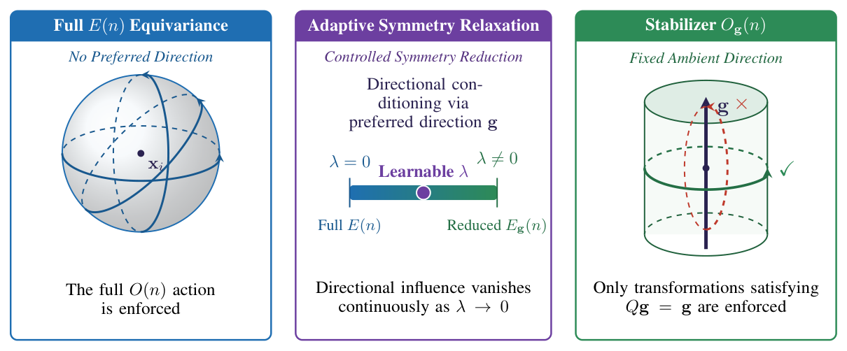
Every section so far has worked to earn an exact guarantee; the paper’s other centrepiece asks when to give part of it back. Full \(E(n)\)-equivariance is the right prior only when the physics has no preferred direction. Gravity, background flow, an applied field, all select an axis and reduce the true symmetry group. Hard-coding the reduction (as subequivariant GNNs do) requires knowing the axis; ignoring it wastes the information. ESNN answers with one scalar: symmetry becomes a dial rather than a switch, and the dial starts at zero.
When symmetry relaxation is enabled, the edge context is augmented with a single signed projection,
where \(\mathbf{g}\) is a global preferred direction, prescribed, or a learned parameter, and \(\lambda_g\) is a learnable relaxation coefficient initialised at zero. (Two disambiguations. First: \(\lambda_g\) is one scalar per layer, with \(\mathbf{g}\) shared across all layers, and has nothing to do with the per-edge transport scale \(\lambda_{ij}\). Second: \(\mathbf{g}\in\mathbb{R}^n\) is a direction, not the channel gate \(\mathbf{g}_{ij}\).) Theorem 6.1 gives the exact accounting. For \(\lambda_g\neq 0\), the architecture is equivariant to the stabiliser subgroup \(E_{\mathbf{g}}(n)=O_{\mathbf{g}}(n)\ltimes\mathbb{R}^n\), all translations, plus every rotation or reflection fixing \(\mathbf{g}\). The reason is one line: \(\langle Q\mathbf{r},\mathbf{g}\rangle=\langle\mathbf{r},\mathbf{g}\rangle\) exactly when \(Q^{\top}\mathbf{g}=\mathbf{g}\). And at \(\lambda_g=0\) the directional term vanishes identically, so full \(E(n)\)-equivariance is recovered, not approximately, exactly.
Where transport earns its keep
The design decisions above are testable claims, and the evaluation tests them one at a time: four questions, each isolating one.
Q1, Does richer transport help when full symmetry is correct? Charged 5-body dynamics in the reduced-data protocol, 3,000 training trajectories, predicting 0.2 simulation-time units ahead. Here \(E(3)\) is the true prior, so EGNN and ESNN share the same symmetry assumption and differ only in transport; the question is transport at a fixed symmetry class, not state of the art on the benchmark.
| Method | MSE ↓ |
|---|---|
| SE(3)-Transformer | 0.0244 |
| Tensor Field Network | 0.0155 |
| Graph Neural Network | 0.0107 |
| EGNN | 0.0071 |
| ESNN-Id | 0.0060 |
| ESNN-Diag | 0.0054 |
| ESNN-RadTan | 0.0052 |
| ESNN-Ortho | 0.0051 |
Every variant beats EGNN; the best cuts error by ~28%. The instructive gap is Id → Ortho/RadTan: the architecture shell explains part of the gain (0.0071 → 0.0060), but learning the transport itself is worth the rest. Anisotropic edge maps pay even when the symmetry assumption is unchanged.
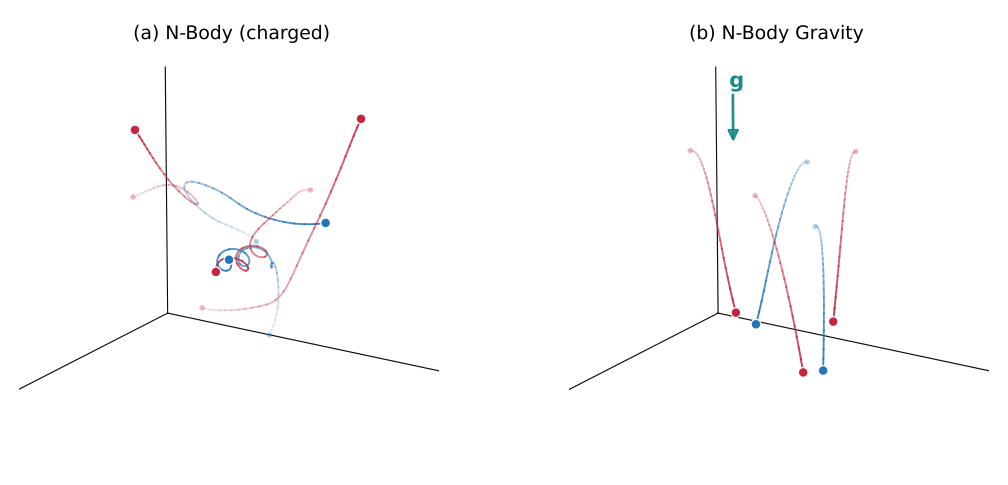
Q2, Can it exploit reduced symmetry, or discover the axis? Same system plus uniform gravity \(\mathbf{a}_g=(0,0,-9.81)^{\top}\), now observed at the very start of the trajectory and predicted over a five-times-longer horizon. The early window is the point of the protocol: run the system long enough and gravity stamps a common downward drift onto every velocity, and since velocities are input vector features, any equivariant model could then read the axis straight off them. Observing before that happens forces the model to infer the hidden axis rather than be handed it. Three matched settings: None (fully equivariant), Fixed (true axis given), Learned (a single trainable global vector, axis inferred from dynamics).
| Mode | MSE ↓ (best transport) | Alignment \(A_g\) ↑ |
|---|---|---|
| None, full \(E(3)\) | 0.1019 ± 0.0324 | – |
| Fixed \(\mathbf{g}\) | 0.0198 ± 0.0017 | 1.000 (by construction) |
| Learned \(\mathbf{g}\) | 0.0197 ± 0.0015 | 1.000 |
A five-fold error gap separates the equivariant model from both relaxed ones, the cost of insisting on a symmetry the data does not have. The result that matters: Learned matches Fixed, with sign-invariant alignment \(\lvert\langle\widehat{\mathbf{g}},\widehat{\mathbf{g}}_{\mathrm{true}}\rangle\rvert=1.000\) across every transport family and seed. Nothing pushes it there: no penalty on \(\mathbf{g}\) or \(\lambda_g\) appears anywhere in the objective, and the equivariant prior lives entirely in the zero initialisation. Yet the learned relaxation scales \(\max_\ell\lvert\lambda^{(\ell)}_g\rvert\lVert\mathbf{g}\rVert_2\) come out decisively non-zero (0.40 ± 0.07 for Ortho, 2.06 ± 0.63 for RadTan).
The zero-initialised pathway switches itself on and points at gravity.
Q3, Does it hold up in mesh-based simulation? Three MeshGraphNets benchmarks: incompressible flow (CylinderFlow), structural deformation (DeformingPlate), compressible aerodynamics (Airfoil).
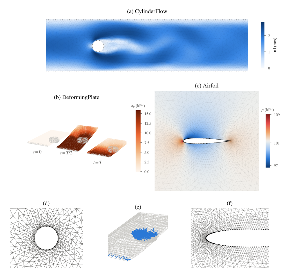
RMSE ×10⁻³ at one step, 50 steps, and full rollout, the model’s own predictions fed back in to the end of the trajectory, MeshGraphNets rows as published by Pfaff et al. (2021):
| System | Model | 1-step ↓ | 50-step ↓ | Full trajectory ↓ |
|---|---|---|---|---|
| DeformingPlate | MeshGraphNets | 0.25 ± 0.05 | 1.8 ± 0.5 | 15.1 ± 4.0 |
| ESNN-RadTan | 0.08 | 1.0 | 5.8 | |
| CylinderFlow | MeshGraphNets | 2.34 ± 0.12 | 6.3 ± 0.7 | 40.88 ± 7.2 |
| ESNN-Ortho | 2.40 | 7.7 | 35.94 | |
| Airfoil | MeshGraphNets | 314 ± 36 | 582 ± 37 | 11529 ± 1203 |
| ESNN-RadTan | 2584 | 3346 | 7787 |
In one line: ESNN wins every column on DeformingPlate and takes the full trajectory on all three systems; MeshGraphNets keeps the short horizons on the two flow tasks.
The paper is candid that the advantage is not uniform, and the pattern is more interesting than a clean sweep would be. On DeformingPlate, where anisotropy is the physics: material response along versus across the deformation, ESNN is better at every horizon, and not only for the best variant. Every ESNN family, Identity included, beats MeshGraphNets at all three horizons, with the best full-rollout error under 40% of the baseline’s. The Q1 audit applies here too: the equivariant shell alone takes 15.1 to 7.7 (ESNN-Id), and radial–tangential anisotropy takes it the rest of the way to 5.8.
CylinderFlow and Airfoil trade short-horizon accuracy for better full-trajectory error, modestly on CylinderFlow (40.88 → 35.94), substantially on Airfoil (11529 → 7787). The trade is steep: Airfoil’s one-step error lands at eight times the baseline’s, and CylinderFlow’s full-rollout gain sits within MeshGraphNets’ reported variance (± 7.2), where DeformingPlate’s and Airfoil’s do not. The suggestion: structured equivariant transport matters most where geometric information must survive repeated propagation through an evolving state, exactly where autoregressive rollouts die. The paper offers the pattern, not a mechanism, so read it as the hypothesis the numbers point to. Still: this is a general-purpose geometric architecture matching a purpose-built mesh simulator on its own benchmarks.
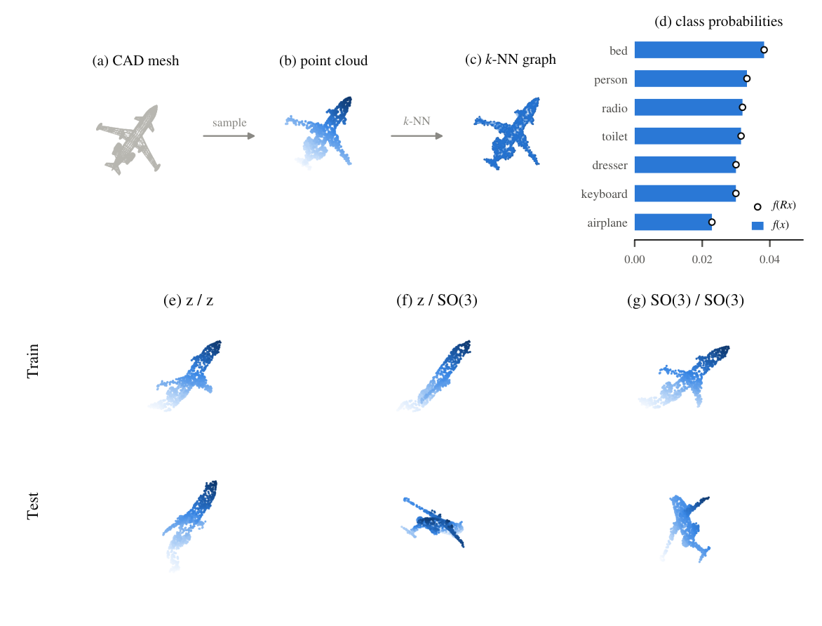
Q4, Does the guarantee transfer off physics? ModelNet40 classification on k-NN graphs, with the informative protocol being \(z/\mathrm{SO}(3)\): train with vertical-axis rotations only, test under arbitrary 3D rotations. Baseline numbers follow Lippmann et al. (2024); \(\Delta_{\mathrm{OOD}}\) is the accuracy drop from z/z to z/SO(3), how much a model loses on orientations never seen in training (protocol names read train/test).
| Method | z/z | z/SO(3) | SO(3)/SO(3) | \(\Delta_{\mathrm{OOD}}\) ↓ |
|---|---|---|---|---|
| PointNet | 85.9 | 19.6 | 74.7 | 66.3 |
| DGCNN | 90.3 | 33.8 | 88.6 | 56.5 |
| VN-DGCNN | 89.5 | 89.5 | 90.2 | 0.0 |
| CRIN | 91.8 | 91.8 | 91.8 | 0.0 |
| ESNN-Id | 84.7 | 85.7 | 85.6 | 1.1 |
| ESNN-Diag | 84.6 | 84.3 | 84.4 | 0.3 |
| ESNN-Ortho | 84.9 | 85.2 | 84.7 | 0.2 |
| ESNN-RadTan | 85.4 | 84.6 | 86.3 | 0.7 |
ESNN holds 84–86% essentially unmoved across protocols (\(\Delta_{\mathrm{OOD}}\le 1.1\), and just 0.2 for Ortho) while orientation-sensitive baselines shed 50+ points; the exactly invariant baselines sit at 0.0 by construction. Exact invariance would put ESNN at 0.0 as well; the residual 0.2–1.1 is run-to-run evaluation noise, not orientation sensitivity, ESNN-Id actually gains a point under rotations it never saw, which no orientation-sensitive model can do. This is robustness by construction, not by augmentation. Specialised rotation-invariant point-cloud architectures do reach higher absolute accuracy; the point of this experiment is transfer, the same transport framework moving from particle physics to shape recognition intact.
QM9, as a coda. On twelve invariant molecular targets, the strongest ESNN variant beats EGNN on nine (including \(\alpha\), \(\Delta\epsilon\), \(\mu\)), with radial–tangential the best family on most, evidence the transport helps even when the final prediction is a single invariant scalar. EGNN keeps \(C_v\), \(H\) and \(\langle R^2\rangle\), and dedicated molecular architectures remain ahead in absolute terms; the paper frames this benchmark as a transport-mechanism test, not a leaderboard entry.
Where this sits in the sheaf story
Three threads of this book meet in ESNN.
The meaning of restriction maps. The recurring finding in this literature, from identity-sheaf baselines being competitive to Conn-NSD computing maps instead of learning them, is that unrestricted learned maps are not automatically useful; structure is what makes them earn their parameters. ESNN is the sharpest version of that lesson so far: it derives the correct structure from a symmetry requirement, and then proves (Theorem 4.3) that under displacement conditioning nothing else was available anyway. The sheaf stops being an abstract algebraic gadget and becomes a carrier of physical transformation law.
Directionality. The self-adjoint sheaf Laplacian’s inability to treat \(i\to j\) and \(j\to i\) differently drove CSNN to directed sheaves; ESNN arrives at directed transport from the opposite motivation, physical interactions are asymmetric, and keeps the classical picture available as an exact specialisation rather than discarding it.
Symmetry as a dial rather than a switch. Where the rest of the sheaf literature fixes its symmetry stance in the architecture, the relaxation mechanism makes it a differentiable, zero-initialised, group-theoretically-accounted parameter. That template, exact equivariance as the origin of a learnable coordinate, stabiliser guarantees away from it, should travel well beyond this paper.
None of which closes the story.
- Features stay scalar-plus-first-order-vector, no higher tensors.
- The completeness theorem covers displacement-conditioned linear transport only; the feature-conditioned class is uncharacterised.
- The relaxation mechanism assumes one global preferred direction, not a spatially varying field.
- The mesh gains are horizon- and system-dependent rather than uniform.
✅ Key Takeaways
- ESNN bridges the two literatures: sheaf-style matrix-valued edge transport, constrained, unlike generic sheaf parameterisations, to respect the ambient Euclidean transformation law of geometric vector features.
- Every transport factorises as covariant spatial operator × invariant channel operator, \(\sum_k \mathbf{S}^{(k)}_{ij}\mathbf{V}_j\mathbf{M}^{(k)}_{ij}\), the symmetry burden lives entirely on the spatial factor, leaving channel mixing free.
- Four families: Identity, Diagonal (isotropic), Orthogonal (feature-conditioned \(SO(n)\) rotation via matrix exponential of a skew cross-feature generator), Radial–Tangential (independent longitudinal/transverse channel maps; projectors applied in \(\mathcal{O}(nc_v)\), the full transport in \(\mathcal{O}(nc_v^2)\)).
- Theorem 4.3: with displacement as the only covariant input, the radial–tangential form is the complete class of linear \(O(n)\)-equivariant transports, proved by a stabiliser/Schur argument. Scope: needs full \(O(n)\) (under \(SO(3)\), \([\widehat{\mathbf{r}}]_{\times}\) sneaks in) and displacement-only conditioning.
- The transport operator is directed and generally not self-adjoint, a quiver representation, with adjoint-consistency and orthogonality recovering classical connection sheaves exactly as a special case.
- Controlled symmetry relaxation via zero-initialised \(\lambda_g\langle\mathbf{r}_{ij},\mathbf{g}\rangle\): exact \(E(n)\)-equivariance at \(\lambda_g=0\), exact stabiliser equivariance \(E_{\mathbf{g}}(n)=O_{\mathbf{g}}(n)\ltimes\mathbb{R}^n\) when active, and \(\mathbf{g}\) learnable, recovering the gravity axis from data with alignment 1.000 while matching the oracle given the true axis.
- Results: −28% MSE vs EGNN on charged N-body; 5× error reduction under gravity vs the fully equivariant model; DeformingPlate beaten at every horizon (15.1 → 5.8 full-rollout) and best full-trajectory error on all three mesh benchmarks; ModelNet40 accuracy shifting ≤ 1.1 points under unseen test rotations.
- Limits, plainly stated: first-order features only, completeness restricted to displacement conditioning, one global preferred direction, and mesh gains concentrated at long horizons.
References
- Borgi, A.*, Severino, M.*, Silvestri, F., & Liò, P. (2026). Equivariant Sheaf Neural Networks: Learning Geometric Transport on Graphs. arXiv:2608.28853.
- Satorras, V. G., Hoogeboom, E., & Welling, M. (2021). E(n) Equivariant Graph Neural Networks. ICML 2021.
- Hansen, J., & Gebhart, T. (2020). Sheaf Neural Networks. NeurIPS 2020 Workshop on TDA and Beyond.
- Bodnar, C., Di Giovanni, F., Chamberlain, B. P., Liò, P., & Bronstein, M. M. (2022). Neural Sheaf Diffusion: A Topological Perspective on Heterophily and Oversmoothing in GNNs. NeurIPS 2022.
- Barbero, F., Bodnar, C., Sáez de Ocáriz Borde, H., Bronstein, M., Veličković, P., & Liò, P. (2022). Sheaf Neural Networks with Connection Laplacians. ICML 2022 TAG-ML Workshop.
- Ribeiro, A., Tenório, A. L., Belieni, J., Souza, A. H., & Mesquita, D. (2025). Cooperative Sheaf Neural Networks. arXiv:2507.00647.
- Fiorini, S., Aktas, H., Duta, I., Coniglio, S., Morerio, P., Del Bue, A., & Liò, P. (2025). Sheaves Reloaded: A Directional Awakening. arXiv:2506.02842.
- Hajij, M., et al. (2025). Copresheaf Topological Neural Networks: A Generalized Deep Learning Framework. NeurIPS 2025.
- Han, J., Huang, W., Ma, H., Li, J., Tenenbaum, J., & Gan, C. (2022). Learning Physical Dynamics with Subequivariant Graph Neural Networks. NeurIPS 2022.
- Hofgard, E., Wang, R., Walters, R., & Smidt, T. (2024). Relaxed Equivariant Graph Neural Networks. arXiv:2407.20471.
- Schütt, K., Unke, O., & Gastegger, M. (2021). Equivariant Message Passing for the Prediction of Tensorial Properties and Molecular Spectra (PaiNN). ICML 2021.
- Jing, B., Eismann, S., Soni, P. N., & Dror, R. O. (2021). Equivariant Graph Neural Networks for 3D Macromolecular Structure. arXiv:2106.03843 (GVP).
- Thomas, N., Smidt, T., Kearnes, S., Yang, L., Li, L., Kohlhoff, K., & Riley, P. (2018). Tensor Field Networks. arXiv:1802.08219.
- Fuchs, F. B., Worrall, D. E., Fischer, V., & Welling, M. (2020). SE(3)-Transformers: 3D Roto-Translation Equivariant Attention Networks. NeurIPS 2020.
- Pfaff, T., Fortunato, M., Sanchez-Gonzalez, A., & Battaglia, P. W. (2021). Learning Mesh-Based Simulation with Graph Networks. ICLR 2021.
- Kipf, T., Fetaya, E., Wang, K.-C., Welling, M., & Zemel, R. (2018). Neural Relational Inference for Interacting Systems. ICML 2018.
- Wu, Z., Song, S., Khosla, A., Yu, F., Zhang, L., Tang, X., & Xiao, J. (2015). 3D ShapeNets: A Deep Representation for Volumetric Shapes. CVPR 2015.
- Lippmann, P., Gerhartz, G., Remme, R., & Hamprecht, F. A. (2024). Beyond Canonicalization: How Tensorial Messages Improve Equivariant Message Passing. arXiv:2405.15389 (source of the ModelNet40 baseline comparison).
- Hansen, J., & Ghrist, R. (2019). Toward a Spectral Theory of Cellular Sheaves. Journal of Applied and Computational Topology, 3(4), 315–358.