
PolyNSD: Polynomial Neural Sheaf Diffusion
Published:
Why This Paper Exists
PolyNSD starts from a practical frustration: Neural Sheaf Diffusion is powerful, but it is harder to train and scale than it should be. The original formulation asks the model to repeatedly build and normalise a sheaf diffusion operator with dense restriction maps and expensive matrix machinery. That is a strong theoretical framework, but not always a friendly engineering one.
This paper asks a sharper question: can we keep the geometric benefits of sheaf diffusion while making the propagation rule behave more like a stable, interpretable spectral GNN?
Background: Neural Sheaf Diffusion
A Sheaf Neural Network enriches a graph with a cellular sheaf: each node and edge gets a vector space (a stalk), and each endpoint of each edge gets a restriction map encoding how node signals relate to edge signals. The sheaf Laplacian encodes this relational geometry and replaces the standard graph Laplacian in the diffusion operator.
Neural Sheaf Diffusion (NSD), the dominant sheaf GNN approach, learns restriction maps end-to-end and runs diffusion on the sheaf Laplacian. It handles heterophily well and resists oversmoothing, but has three practical problems:
- SVD-based normalisation: requires expensive SVD decomposition of the sheaf Laplacian at every layer, making Laplacian rebuilds slow.
- Dense restriction maps: one \(d \times d\) matrix per node-edge pair, scaling quadratically with stalk dimension \(d\).
- Brittle gradients: the normalised sheaf Laplacian construction is numerically unstable for large \(d\), leading to gradient issues.
The Main Design Choice
PolyNSD takes the perspective of spectral GNNs seriously: instead of repeatedly applying a fragile diffusion operator layer after layer, it learns a polynomial filter directly on the normalised sheaf Laplacian. That means the network can shape the frequency response explicitly, while keeping the computation sparse and stable.
The PolyNSD Fix
PolyNSD replaces the NSD propagation operator with a degree-\(K\) polynomial of a spectrally rescaled normalised sheaf Laplacian, evaluated via a stable three-term Chebyshev recurrence.
This gives:
- Explicit \(K\)-hop receptive field in a single layer (independently of the stalk dimension \(d\)).
- Trainable spectral response as a convex mixture of \(K+1\) orthogonal polynomial basis responses, the model learns which frequency components to amplify or suppress.
- No SVD needed: the recurrence only requires sparse matrix-vector products.
- Stability via convex mixtures (coefficients sum to 1) + spectral rescaling to \([-1, 1]\) + residual/gated paths.
Architecture Overview
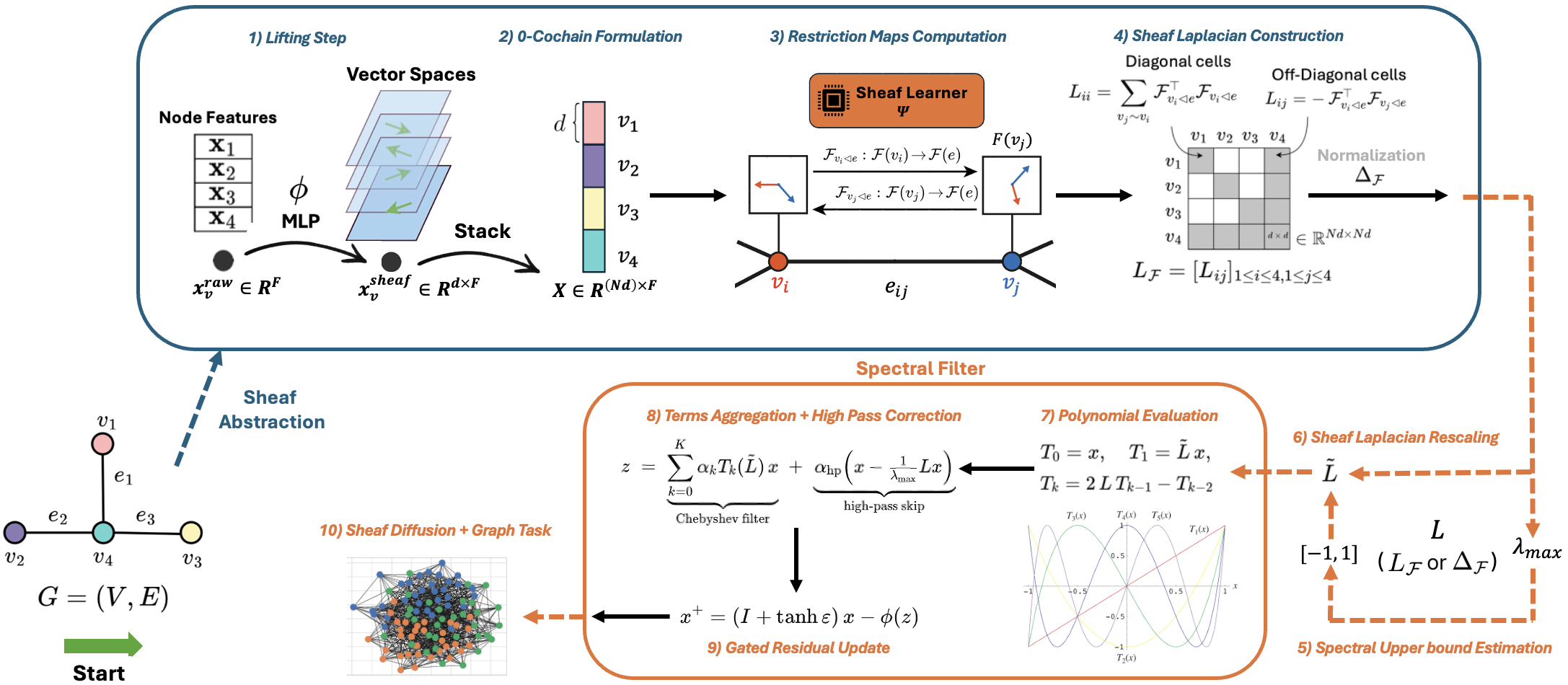
The full architecture is deliberately clean. Node features are lifted into stalk spaces, diffusion is performed through polynomial filtering on the sheaf Laplacian, and the output head reads the result back for prediction. That simplicity is part of the contribution: the model becomes easier to reason about than earlier sheaf pipelines with heavier normalisation machinery.
Diagonal Restriction Maps
The key parameter-reduction insight: diagonal restriction maps (a vector of \(d\) scalars per node-edge pair instead of a \(d \times d\) matrix) are sufficient for strong performance. This reduces per-edge parameter count from \(O(d^2)\) to \(O(d)\) and decouples performance from large stalk dimensions.
The Practical Win
This is where the paper becomes especially useful. Many sheaf models implicitly suggest that more expressive geometry requires larger dense restriction maps. PolyNSD shows that this is often the wrong tradeoff. If the spectral filter is doing the right global work, the local maps can stay lightweight and still capture the anisotropic behavior that matters.
Why Diagonal Maps Are Enough
This is one of the paper’s most useful empirical findings. Earlier sheaf models tended to assume that expressive sheaf learning required large dense restriction matrices. PolyNSD shows that this is often unnecessary: once the spectral filter itself is strong enough, diagonal maps can already encode the right anisotropic behaviour while being much cheaper to train and much less numerically delicate.
Concrete 3-Node Chebyshev Recurrence Example
Consider a path graph A–B–C with \(d = 1\) stalks (scalar features) and diagonal restriction maps. Let \(\mathcal{F}_{A \trianglelefteq e_{AB}} = \operatorname{diag}(1) = 1\), \(\mathcal{F}_{B \trianglelefteq e_{AB}} = \operatorname{diag}(-1) = -1\) on edge \(AB\), and \(\mathcal{F}_{B \trianglelefteq e_{BC}} = \operatorname{diag}(1) = 1\), \(\mathcal{F}_{C \trianglelefteq e_{BC}} = \operatorname{diag}(1) = 1\) on edge \(BC\). Initial node features: \(x = [\,x_A,\ x_B,\ x_C\,]^{\top}\).
Step 1, Build the sheaf Laplacian block. For a path A–B–C with these maps, the (unnormalised) sheaf Laplacian is:
- Row \(A\): contribution from edge \(AB\): \(\mathcal{F}_{A}^{\top}\mathcal{F}_{A} - \mathcal{F}_{A}^{\top}\mathcal{F}_{B} = 1 \cdot I - 1 \cdot (-1) = 2\) on diagonal \(A\).
- Row \(B\): \(B\) is incident to both edges.
- Row \(C\): \(C\) is incident to edge \(BC\) only.
After spectral rescaling to \([-1, 1]\) (dividing by the largest eigenvalue ~3 and shifting), we get the normalised \(\tilde{\Delta}_{\mathcal{F}}\).
Step 2, Chebyshev recurrence with \(K = 2\). The three Chebyshev basis evaluations are:
Step 3, 3-hop receptive field “for free”. The \(T_2\) term gives node A access to information from node C (2 hops away) in a single PolyNSD layer with \(K = 2\). In NSD, reaching C from A requires 2 separate message-passing layers (A→B in layer 1, B→C in layer 2). PolyNSD achieves the same 2-hop receptive field in one layer, because the Chebyshev recurrence computes multi-hop aggregations algebraically without stacking layers. For \(K = 3\), node A would see 3 hops with a single filter evaluation. This is the key efficiency gain: \(K\) polynomial terms in one layer = \(K\) separate NSD layers, but with only one set of learned parameters and one set of map computations.
Learned weights example. With \(K = 2\), PolyNSD learns weights \([\alpha_0, \alpha_1, \alpha_2]\) (convex mixture summing to 1). For a homophilic graph, the model might learn \([0.6, 0.3, 0.1]\) (low-pass, dominated by \(T_0\)). For a heterophilic graph like Cornell, it might learn \([0.1, -0.3, 0.6]\) (high-pass, dominated by \(T_2\) which oscillates, amplifying differences between nodes). This spectral flexibility is what makes PolyNSD work well on both homophilic and heterophilic benchmarks with a single architecture.
Results
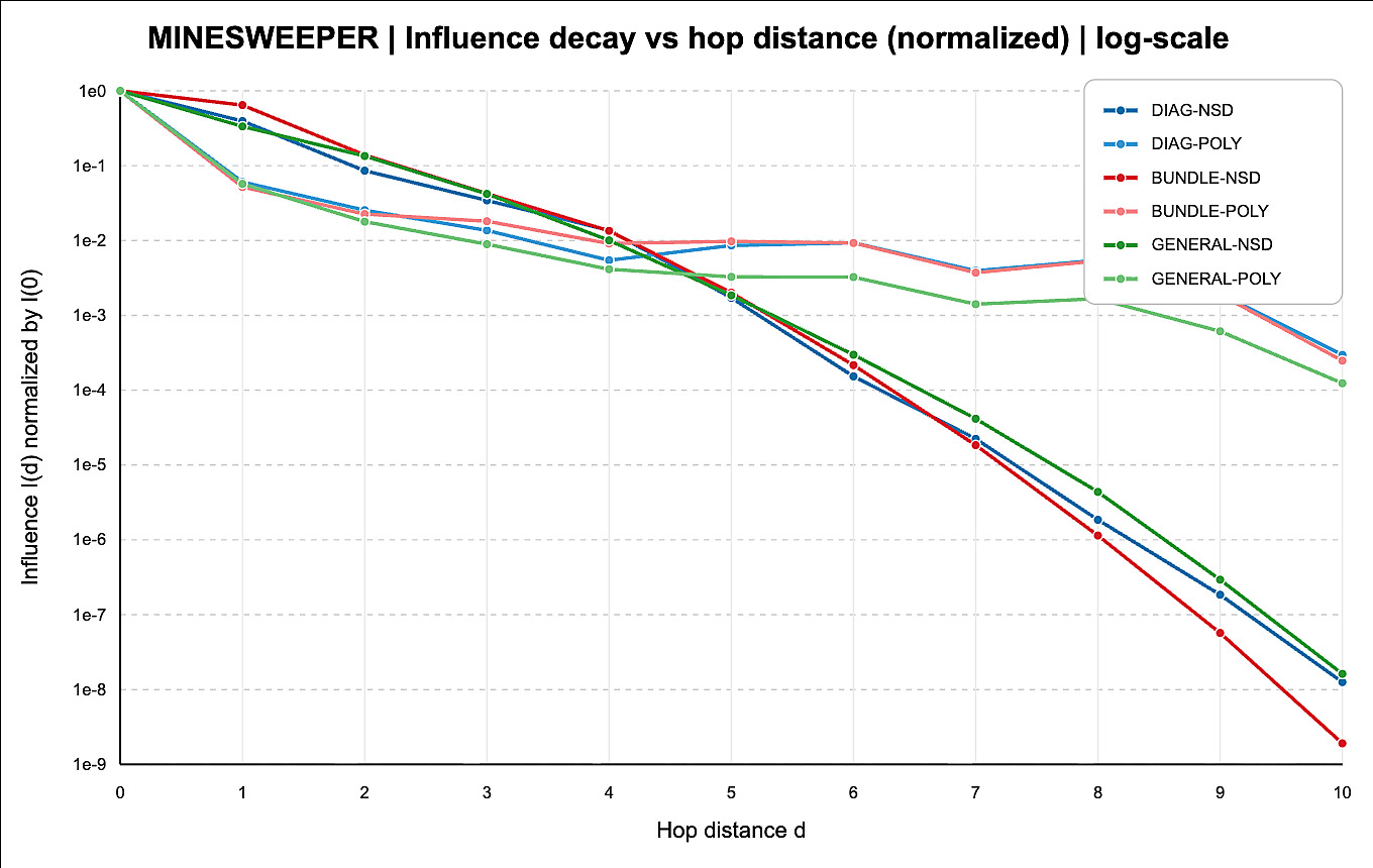
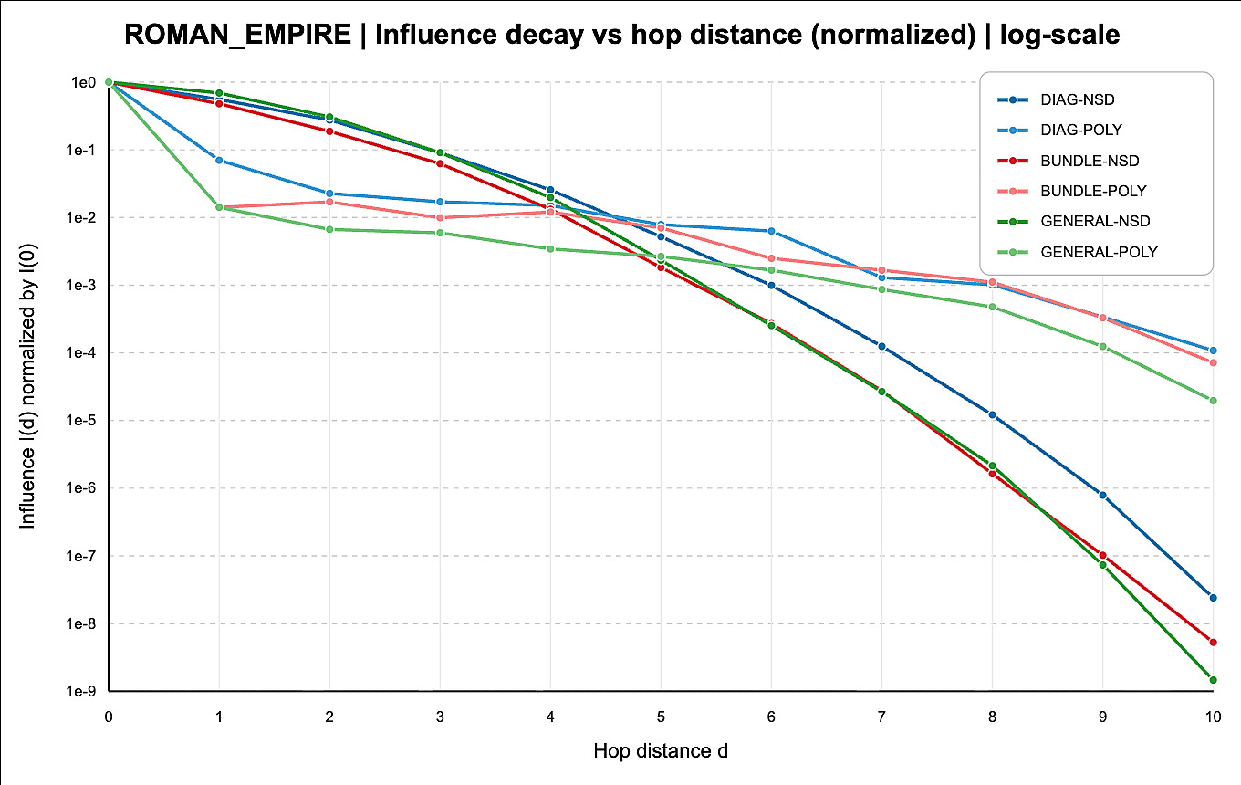
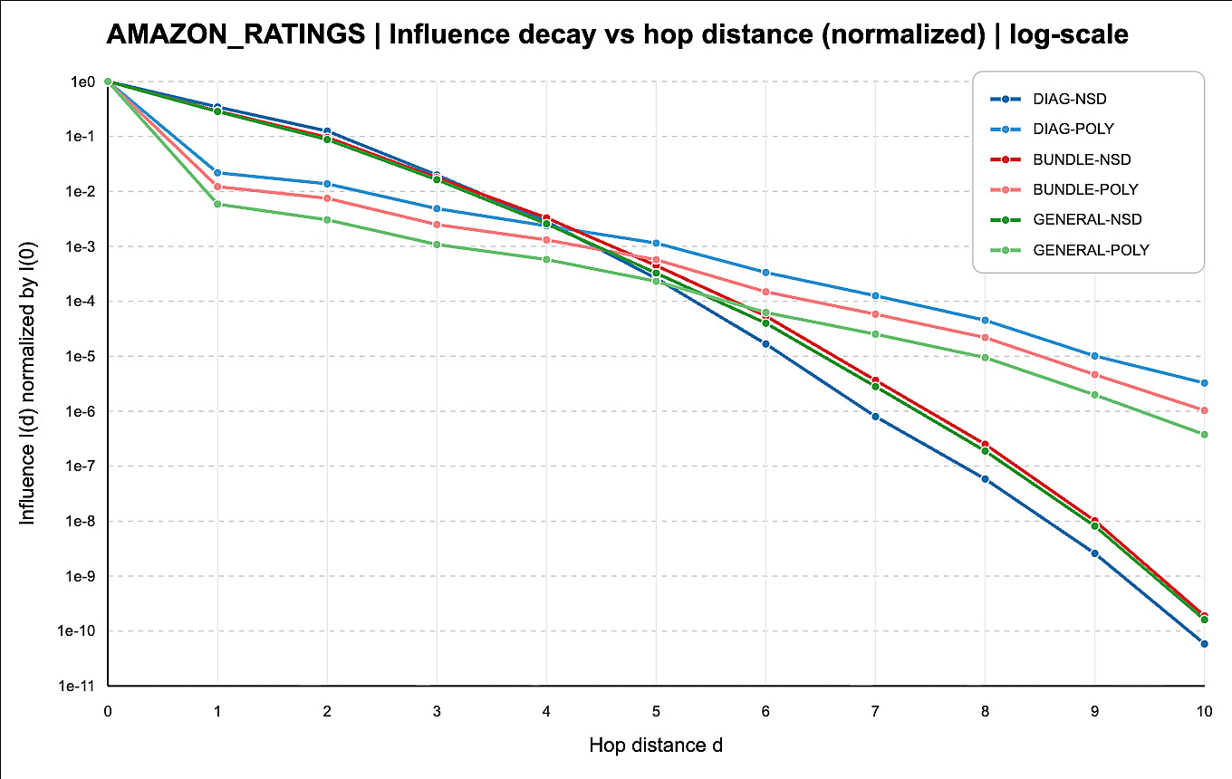
Key results vs. NSD and spectral GNN baselines:
- New SOTA on both homophilic (Cora, CiteSeer, PubMed) and heterophilic (Texas, Film, Wisconsin) benchmarks, inverting the NSD trend that required large stalk dimensions for heterophilic gains.
- Diagonal maps + small d match or exceed NSD with dense maps + large d.
- Lower runtime and memory: no SVD, sparse recurrence, small stalk dimensions.
- Spectral filter shape is interpretable: the model learns when to apply low-pass (homophilic) vs. high-pass (heterophilic) filters.
Why the Result Is Interesting Beyond This Paper
PolyNSD is more than a performance bump over NSD. It suggests a better recipe for future sheaf models: keep the geometric inductive bias, but move expensive expressivity away from fragile local parameterisations and into stable global filtering mechanisms. That is a useful design lesson whether the next step is node classification, heterophily, or more general geometric deep learning.
Why This Paper Matters
PolyNSD is important because it makes sheaf GNNs more usable. It preserves the geometric advantages of sheaf diffusion, but removes several implementation bottlenecks that previously made these models expensive or unstable. In practice, that is what turns a promising theory into something researchers can run, compare, and build on.
✅ Key Takeaways
- PolyNSD replaces the NSD diffusion operator with a degree-\(K\) Chebyshev polynomial in the normalised sheaf Laplacian, evaluated via a stable three-term recurrence.
- Diagonal restriction maps are sufficient, decoupling performance from stalk dimension and reducing parameters from \(O(d^2)\) to \(O(d)\) per edge.
- Stable by design: convex mixture coefficients + spectral rescaling + residual paths prevent gradient collapse.
- SOTA on homo- and heterophilic benchmarks with lower runtime and memory than NSD.