Modern Activation Functions: GELU, SiLU, Mish, and Smooth Gating

10 minute read

Published:

TL;DR: Modern activations try to keep the optimization benefits of ReLU while making the transition around zero smoother and more expressive. GELU became standard in Transformers, SiLU/Swish became popular in efficient deep networks, and Mish explored even more flexible smooth non-monotonic behavior.

Why ReLU Was Not the End of the Story

Intuition First: Think of ReLU as a light switch — it is either fully off or fully on. That simplicity is great for optimization, but sometimes you want a dimmer switch: something that smoothly transitions from "mostly off" to "fully on," with a meaningful response even near zero. Modern activations are dimmers. They keep the same "pass positives strongly" behavior of ReLU while giving the network richer structure near the transition point.

ReLU solved a huge optimization problem, but it also introduced a blunt shape:

  • exactly zero on the negative side
  • exactly linear on the positive side
  • non-differentiable at zero

That simplicity is often a strength, but it is not always the best match for large modern architectures. Once deep learning scaled up, researchers started testing smoother alternatives that preserve gradient flow while making the network’s response less abrupt.

The Main Modern Idea

Instead of saying:

\[ f(x) = \begin{cases} 0, & x < 0 \\ x, & x \ge 0 \end{cases} \]

modern activations often say:

\[ f(x) \text{ should turn on smoothly and keep a useful derivative near } x = 0 \]

That makes them feel more like soft gates than hard thresholds.
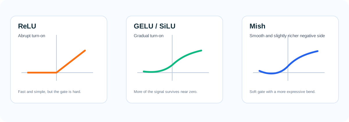
Diagram comparing a hard ReLU switch with smoother GELU, SiLU, and Mish style gating
Figure 1 — Modern activations are easier to understand if you think in terms of gating. ReLU flips on abruptly, while GELU, SiLU, and Mish let the signal turn on gradually and keep more structure around zero.

Smooth ReLU-Like Families

ELU, SELU, and CELU

These functions keep the positive linear branch, but replace the dead negative side with a smooth saturating tail.

  • ELU: negative values bend toward a negative plateau
  • SELU: a self-normalizing variant designed to stabilize mean and variance
  • CELU: a continuously differentiable ELU-like variant

They are especially interesting because they acknowledge that “all negatives become zero” is sometimes too crude.

Key Insight — why a negative floor helps: ReLU neurons that receive consistently negative input produce zero output and zero gradient — they are effectively dead. ELU solves this by letting negative inputs produce a small but non-zero output (approaching −α ≈ −1). This creates a negative mean activation that pushes subsequent layers to self-correct, reducing the need for careful initialization. SELU takes this further by choosing α and the scale λ analytically (λ≈1.0507, α≈1.6733) so that the activations' mean and variance automatically stay near (0, 1) across layers — a built-in batch-norm effect at no extra computation cost.

GELU

GELU is the activation you now see everywhere in Transformers.

\[ \operatorname{GELU}(x) \approx x \, \Phi(x) \]

where Φ(x) is the Gaussian cumulative distribution function.

The intuition is elegant: instead of passing all positive signals and rejecting all negative ones, GELU keeps a value in proportion to how likely it is to be useful under a Gaussian view of the input.

Key Insight: GELU can be read as "stochastic ReLU." If neuron inputs are roughly Gaussian, then Φ(x) is the probability that a standard normal sample is less than x. So GELU(x) = x · P(keep this value) — it applies a data-driven soft gate. At x=0, exactly half the signal is gated through. At x=2, roughly 97% passes. At x=−2, only 3% passes. Unlike ReLU, even mildly negative values contribute a small residual signal.

Step-by-step numerical comparison — GELU vs. ReLU vs. ELU at key input values:

xReLUELU (α=1)GELUGELU′
−30−0.950−0.0040.020
−10−0.632−0.1590.083
00000.500
1110.8411.083
2221.9551.086
3332.9961.010

Notice how GELU preserves a small negative output near x=−1 (−0.159), giving gradients a foothold even in the mildly negative region — something ReLU completely discards.

Swish and SiLU

\[ \operatorname{SiLU}(x) = x \, \sigma(x) \]

Swish is the same family idea; SiLU is the most common fixed version. These activations are smooth, slightly non-monotonic, and behave like a gated linear response.

Key Insight: SiLU = x · σ(x) has a beautiful interpretation: the sigmoid term acts as a learned data-driven gate on the identity term. When x is large and positive, σ(x)→1 so SiLU behaves like identity. When x is large and negative, σ(x)→0 so SiLU suppresses — but smoothly. The slight dip below zero near x≈−1.28 (SiLU minimum ≈ −0.278) gives the network a small negative anchor, which empirically helps optimization.

Mish

Mish pushes the same logic further:

\[ \operatorname{Mish}(x) = x \, \tanh(\operatorname{softplus}(x)) \]

It is smooth, non-monotonic, and often visually looks like “a softer Swish with a richer negative-side bend.”

Key Insight: Mish wraps SiLU's gating idea inside a tanh, which compresses the gate values into (−1, 1) before scaling by x. The result is unbounded above (like ReLU/SiLU), bounded-below (minimum ≈ −0.31), and has continuous higher-order derivatives. The richer curvature near zero gives optimizers more informative local slope information to work with.

Worked example — tracing a value through SiLU vs GELU vs Mish:

Let x = −0.5 (a mildly negative pre-activation):

FunctionComputationOutputGradient at x=−0.5
ReLUmax(0, −0.5)00 (dead!)
GELU−0.5 · Φ(−0.5) ≈ −0.5 · 0.309−0.154≈ 0.154
SiLU−0.5 · σ(−0.5) ≈ −0.5 · 0.378−0.189≈ 0.072
Mish−0.5 · tanh(softplus(−0.5)) ≈ −0.5 · 0.393−0.196≈ 0.065

All three modern activations preserve a small but non-zero gradient where ReLU goes completely silent.
ELU \[ \operatorname{ELU}(x) = \begin{cases} x, & x > 0 \\ \alpha(e^x - 1), & x \le 0 \end{cases} \]
GELU \[ \operatorname{GELU}(x) \approx \frac{x}{2}\left(1 + \tanh\!\Big(\sqrt{\frac{2}{\pi}}\big(x + 0.044715x^3\big)\Big)\right) \]
Swish / SiLU \[ \operatorname{Swish}(x) = x \, \sigma(\beta x), \qquad \operatorname{SiLU}(x) = x \, \sigma(x) \]
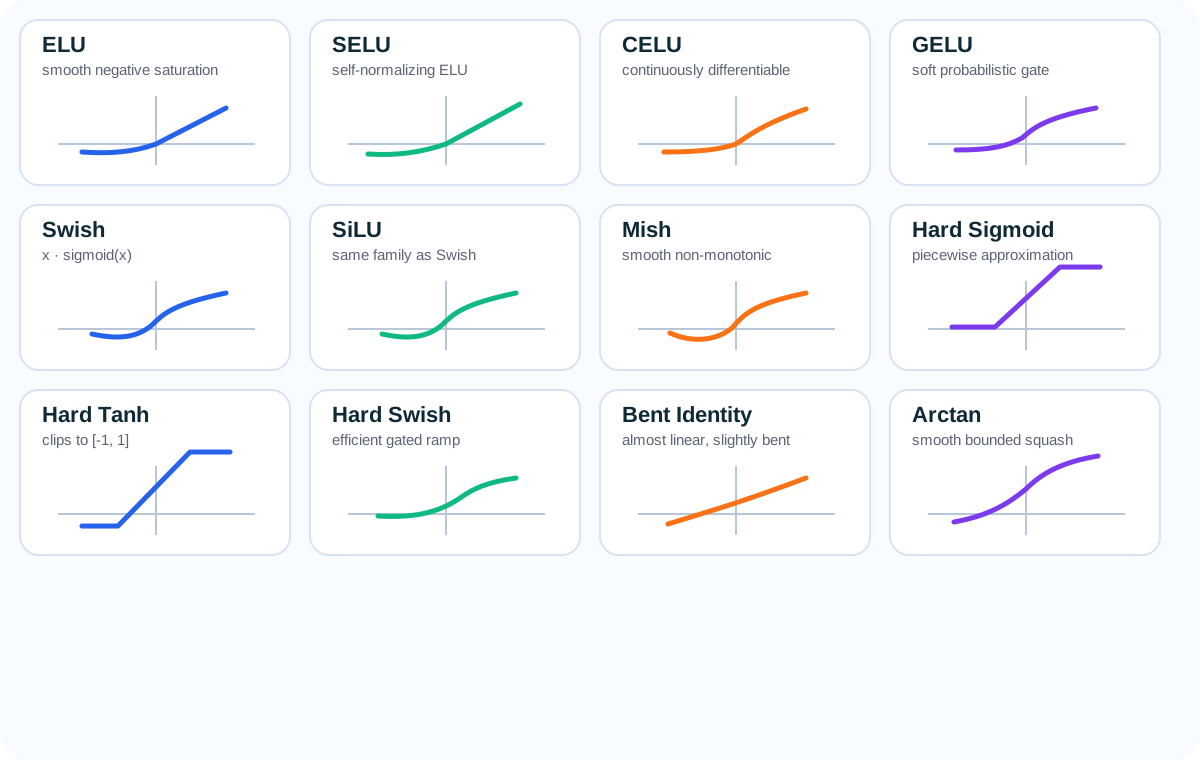
Grid of modern activation functions including ELU, SELU, CELU, GELU, Swish, SiLU, Mish, Hard Sigmoid, Hard Tanh, Hard Swish, Bent Identity, and Arctan
Figure 2 — Modern activation functions mostly differ in one place: how sharply or smoothly they transition around zero, and how much negative information they preserve. GELU, SiLU, and Mish are all trying to replace a hard switch with a softer gate.
−2 −1 0 1 2 1 2 0 ReLU ELU GELU SiLU Mish
Animated overlay — ReLU, ELU, GELU, SiLU, and Mish on the same axes, drawn in sequence. The key region to watch is x ∈ [−2, 0]: ReLU is flat at zero (dead zone), ELU saturates to a fixed floor, while GELU/SiLU/Mish all preserve a smooth negative dip that carries gradient information back through the network.

Fast Approximations and Mobile-Friendly Variants

Smooth functions can be strong, but they are more expensive than piecewise-linear ones. That is why approximation-based activations became popular in efficient models:

  • Hard Sigmoid: piecewise-linear approximation of sigmoid
  • Hard Tanh: clipped tanh-like shape
  • Hard Swish: approximation of Swish used in mobile models

The guiding tradeoff is simple: give up a bit of smoothness to gain speed.

−3 −2 −1 0 1 2 3 SiLU (smooth) Hard Swish (approx.)
SiLU (solid orange) vs. Hard Swish approximation (dashed blue). Hard Swish clips to zero below x=−3, uses the piecewise formula x(x+3)/6 in the middle range, and becomes linear above x=3. The two curves are nearly identical in the critical region [−1, 1] — close enough that mobile networks accept the tradeoff for substantially faster on-device computation.

A Few More Interesting Curves

The visual grid also includes a few less standard but conceptually useful shapes:

  • Bent Identity: almost linear, but gently nonlinear near zero
  • Arctan: another smooth bounded squash
  • SELU / CELU: reminders that negative values do not have to be thrown away completely

These are not the default choices in modern LLMs, but they help build the reader’s intuition: activation design is really about deciding what should happen around zero, in the tails, and in the derivative.

Which Ones Actually Matter Most Today?

ActivationWhy people use itMain tradeoff
GELUVery strong default in TransformersMore expensive than ReLU
SiLU / SwishSmooth, gated, stable, often great in efficient deep netsStill more expensive than ReLU
MishFlexible smooth non-monotonic responseLess standard in large production stacks
Hard SwishGood hardware-friendly approximationLess smooth than the original

Practical Advice

Strong modern defaults:
  • Transformers: GELU remains the standard baseline.
  • Efficient CNNs / mobile models: Hard Swish or SiLU are common.
  • General-purpose modern MLPs: ReLU is still a valid baseline, but SiLU is worth testing.

What Can Go Wrong with Modern Activations?

ActivationPotential problem
ELU / SELU / CELUMore expensive than ReLU and more sensitive to architectural assumptions than many beginners expect.
GELUExcellent in Transformers, but often unnecessary overhead in smaller or simpler models.
SiLU / SwishSmoother optimization, but still costlier than piecewise-linear activations.
MishCan work well, but is less standardized and not always worth the extra complexity.
Hard approximationsFaster on-device, but they give up part of the smooth behavior that motivated the original function.

Common Misunderstanding

The best activation is not the one with the fanciest formula. It is the one whose shape matches:

  1. the optimization constraints,
  2. the architecture,
  3. the hardware budget,
  4. the role of that layer inside the model.

That is why ReLU still survives, GELU dominates Transformers, and Hard Swish shows up in mobile networks. The “best” activation is context-dependent.

Key Insight — the convergence story: GELU, SiLU, and Mish are all smooth approximations of the same underlying idea: a data-dependent soft gate applied to the linear pre-activation. They differ mainly in how they compute the gate (Gaussian CDF, sigmoid, or tanh∘softplus) and in the precise shape of the negative dip. In practice, the differences between them are usually smaller than the difference between any of them and plain ReLU. If you are unsure, GELU for Transformers and SiLU for convolutional/MLP architectures is a well-validated starting point.

References

  1. Hendrycks, D. and Gimpel, K. “Gaussian Error Linear Units (GELUs).” 2016.
  2. Ramachandran, P., Zoph, B., and Le, Q. V. “Searching for Activation Functions.” 2017.
  3. Misra, D. “Mish: A Self Regularized Non-Monotonic Activation Function.” 2019.
  4. Klambauer, G. et al. “Self-Normalizing Neural Networks.” NeurIPS 2017.