
Bochner–Weitzenböck for Sheaves: Transport, Curvature, and What Networks Learn
Published:
Authors: Francesco Maria Guadagnuolo, Alessio Borgi, Dorina Thanou, Pietro Liò.
Preprint: arXiv:2610.28455, submitted 20 October 2026 · PDF, v1.
Implementation: the manuscript builds on the original Neural Sheaf Diffusion code and states that the full experimental code will be released upon acceptance.
In plain words: a sheaf network learns both how neighbouring nodes translate one another’s messages and how strongly different directions matter. This paper opens up that learned operator. One part describes communication across the graph; the other records the local response left after accounting for that communication. The split provides mathematics for understanding the operator and measurements for studying what training actually produces.
From what a sheaf can represent to what training learns
The Sheaf Neural Networks overview introduces restriction maps: each endpoint of an edge transforms its state into a common edge space. Agreement is checked there, rather than by demanding that the original node vectors be identical.
That gives sheaf models a rich representation space. But representational capacity leaves an empirical question unanswered: which part of that space does a particular learning procedure reach? A model can, in principle, represent many sheaves while its optimizer repeatedly favours a much narrower family.
The paper approaches this question through the learned Laplacian itself. It develops a decomposition first, proves what its parts mean, and then turns those parts into diagnostics. The experimental contribution is an analysis of trained networks; it does not introduce a replacement architecture and claim a new accuracy leaderboard.
The starting point: disagreement after transport
Let every stalk have dimension (d). On an edge (e=(v,u)), write the restriction maps as (R_{ve}) and (R_{ue}). For a stacked node signal (x), the sheaf Laplacian (L_{\mathcal F}) has energy
Consequently, its diagonal blocks are sums of (R_{ve}^\top R_{ve}), while the off-diagonal block on an edge is (-R_{ve}^\top R_{ue}). The diagonal measures each endpoint’s own contribution; the off-diagonal encodes how the two endpoints interact.
For an ordinary unsigned graph Laplacian, the diagonal is exactly the sum of the magnitudes of the off-diagonal entries. A general sheaf Laplacian need not satisfy the corresponding block identity. That mismatch is the opening for the decomposition.
The construction also applies beyond node signals. On a complex, the degree-(k) Hodge sheaf Laplacian is
Here (H^k) is sheaf cohomology: the harmonic modes that remain after accounting for local consistency and coboundaries. At degree zero, (H_0=L_{\mathcal F}).
The decomposition: keep the interactions, rebuild the diagonal
For a matrix (A), the paper uses the left matrix absolute value
This is a positive semidefinite matrix, not the entrywise absolute value and not a scalar matrix norm. Its eigenvalues and directions retain information about the strength of an interaction.
Given any symmetric block matrix (H) with equally sized blocks, define
Thus (H=B+F). The Bochner term (B) retains every off-diagonal interaction and replaces the diagonal with the sum of its matrix magnitudes. The Forman term (F) is block diagonal:
Why is (B) positive semidefinite? Take an off-diagonal block (A=U\Sigma V^\top). Its contribution, together with the corresponding diagonal magnitudes, factors as
Summing over pairs proves (B\succeq0). No positivity assumption on (F) is needed for the decomposition to exist. In fact, (F) can have both positive and negative eigenvalues even when the original (H) is a Laplacian and therefore positive semidefinite.
A two-node example you can check by hand
Consider one edge with scalar restriction maps (R_{ve}=2) and (R_{ue}=1). Agreement means (2x_v=x_u). The split is
The Bochner energy is (2(x_v-x_u)^2), which favours equal states. The original energy is ((2x_v-x_u)^2), which favours a different relation. The local term makes up the difference. In continuous diffusion, (\dot x=-Lx=-Bx-Fx), its positive entry damps the first coordinate and its negative entry amplifies the second relative to the Bochner dynamics. The combined system remains governed by the positive semidefinite (L).
The vector ((1,2)^\top) is in (\ker L), but not in (\ker B). This small example shows why we cannot automatically transfer every statement about the Bochner kernel to the full sheaf Laplacian: the Forman term matters.
Bochner matrices: transport with direction-dependent strength
Write an off-diagonal interaction of a Bochner matrix as (B_{vu}=-C_{vu}), and take the polar factorization
The orthogonal factor (W_{vu}) transports from (v) to (u), while (M_{vu}) weights disagreement in the coordinates at (v). Symmetry gives (M_{uv}=W_{vu}M_{vu}W_{vu}^\top). The energy becomes
This unifies several familiar objects:
| Special case | What the edge carries |
|---|---|
| Connection Laplacian | (M_{vu}=w_{vu}I): orthogonal transport with one scalar strength |
| Matrix-weighted Laplacian | (W_{vu}=I): direction-dependent strength without rotation |
| Signed graph, (d=1) | A positive magnitude and a sign, with transport either preserving or reversing the scalar |
| General Bochner matrix | Both orthogonal transport and direction-dependent strength |
For the following kernel, synchronization and random-walk results, the paper assumes block symmetry, invertible nonzero edge interactions and a connected support graph. The basic decomposition itself does not require edge invertibility.
Holonomy determines which states survive
When the edge interactions are invertible, zero energy requires
Orthogonal transport preserves norm, so a Bochner-kernel signal has the same norm at every node of a connected component. Following a closed walk multiplies the edge transports into a holonomy matrix. A surviving signal must return to itself after every such trip.
The kernel therefore has dimension at most (d), and reaches dimension (d) exactly when every closed-walk transport is the identity. Nontrivial holonomy need not eliminate the whole kernel: it may preserve some directions while frustrating others. The radial weights change the cost of disagreement, but, under invertibility, the angular factors determine these exact compatibility conditions.
The normalized Bochner spectrum lies in ([0,2]). The other endpoint, eigenvalue two, is described by the corresponding transport with a sign reversal on every edge: a higher-dimensional version of signed-graph antibalance.
From exact agreement to approximate synchronization
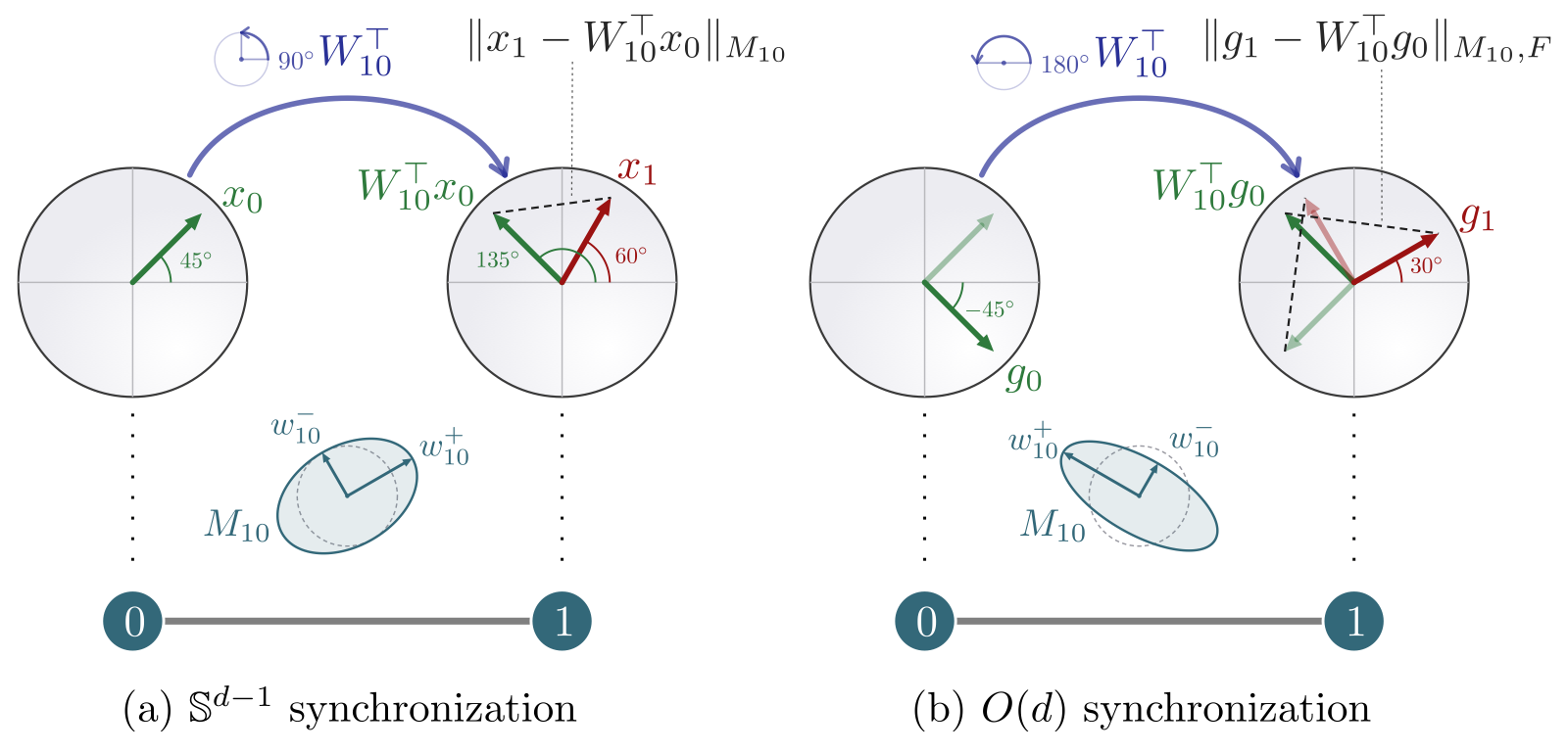
Real systems need not admit perfect agreement. The paper studies three ways to measure the residual mismatch: assign unit vectors to some nodes and let the others abstain; assign a unit vector to every node; or assign a full orthogonal frame to every node.
For the first two, the objective is the generalized Rayleigh quotient
The minima over partial and full assignments are (\eta_G^*) and (\eta_G). These are frustration measures: how much inconsistency remains after choosing the best admissible states?
Let (\kappa_E) be the largest ratio of maximum to minimum eigenvalue of an edge’s (M_{vu}). The partial-synchronization bound is
A low eigenvalue therefore gives a low-frustration assignment, with a penalty for anisotropy. The proof is constructive: use a lowest eigenvector, undo degree normalization, and threshold the node norms before normalizing the retained vectors.
Requiring every node to participate also brings in the connectivity of a scalar companion graph, whose edge weights are (\lambda_{\min}(M_{vu})). Its normalized Laplacian is (\mathcal L_-):
Poor connectivity makes global alignment harder to certify. For full frames, the relevant spectral quantity is the sum of the lowest (d) eigenvalues; the construction uses an isotropized degree and polar projection. These are Cheeger-type results for the Bochner class under the stated assumptions, rather than an unrestricted Cheeger theorem for every sheaf Laplacian.
A random walk that carries an orientation
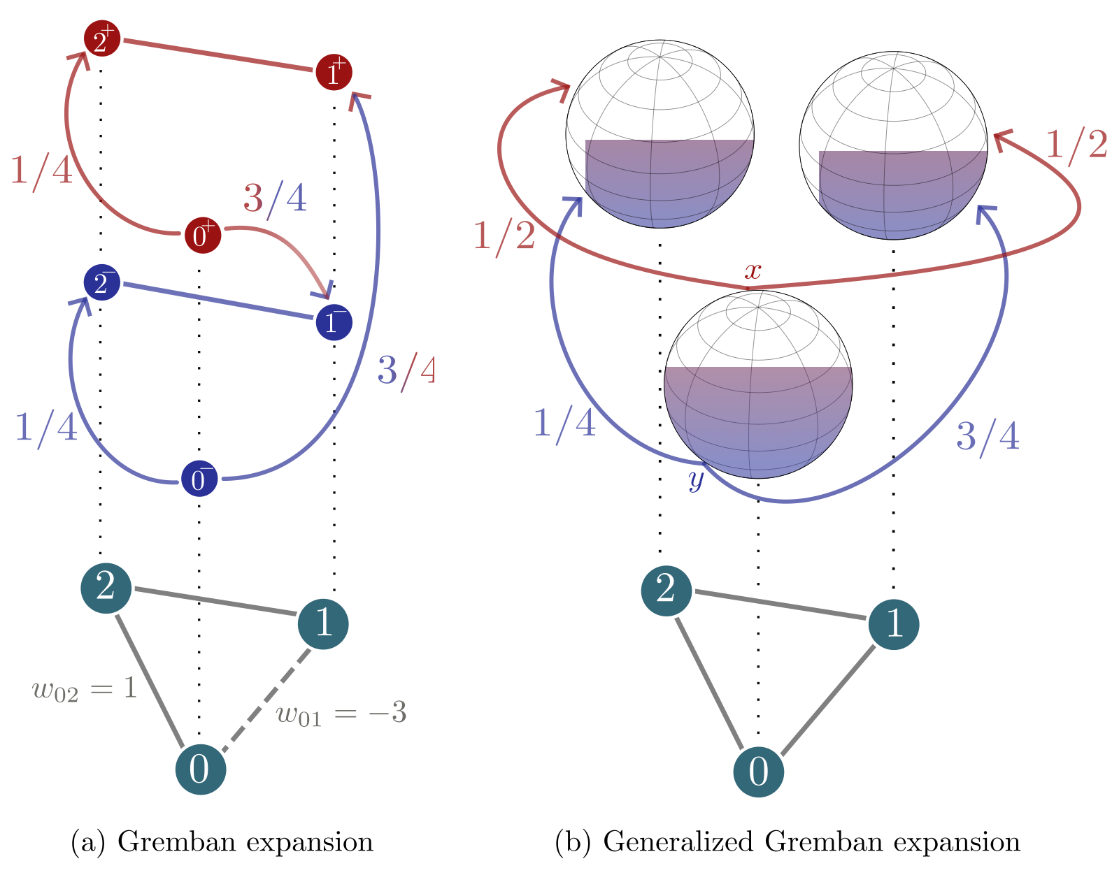
An ordinary random walk remembers its current node. Here the state is a pair ((v,\hat x)), where (\hat x\in S^{d-1}) is a unit vector. Define
Each (P_{vu}) is positive semidefinite and their sum at a node is the identity. The probabilities are therefore nonnegative and sum to one. After choosing (u), the walker updates its orientation deterministically to (W_{vu}\hat x).
For a concrete example, suppose the two outgoing effects are (P_{v1}=\operatorname{diag}(1/2,3/4)) and (P_{v2}=\operatorname{diag}(1/2,1/4)). A walker carrying the horizontal direction chooses either neighbour with probability one half. A vertical orientation gives probabilities three quarters and one quarter. The graph has not changed; the carried direction changes the routing.
If every radial factor is (w_{vu}I), this reduces to the connection-Laplacian walk with scalar transition probabilities. At (d=1), the sphere consists of two signs: crossing a negative edge switches sign, recovering the Gremban expansion.
The walk is attached to the Bochner term. The remaining Forman response must still be accounted for when interpreting the original sheaf diffusion. The paper also notes that this walk is not generally reversible, and leaves the relationship between mixing time and frustration for future work.
Curvature: where the cohomology theorem applies
The decomposition works at every degree, but the term called sheaf Forman Ricci curvature is specifically
Under nonnegative curvature, both summands are positive semidefinite. A harmonic cochain must then lie in both kernels:
This is the bridge from local curvature to global cohomology. With equal-dimensional stalks and invertible restriction maps, the paper proves that a compact connected combinatorial (n)-manifold with nonnegative sheaf Forman curvature satisfies
In arbitrary dimension it gives the bound (dD(M)), where (D(M)) is Forman’s local homological dimension. The proof combines harmonicity with propagation: sufficiently many vanishing values around one vertex force the cochain to vanish everywhere. In the paper’s compact, connected, quasiconvex regular-CW setting, nonnegative curvature everywhere and positive-definite curvature on all edges incident to one vertex force (H^1) to vanish.
These assumptions matter. The theorem is not a claim that any trained graph with a favourable node statistic has small first cohomology. Curvature also depends on the chosen sheaf presentation, and its sign need not agree with that of the underlying complex’s scalar Forman curvature.
Conviction: which nodes does a trained network rely on?
A network carries multiple channels per stalk. At layer (t), node (u) has a matrix (X_t[u]\in\mathbb R^{d\times f_t}). Its conviction is simply
The name comes from opinion dynamics: the norm measures how strongly a state is held. The Bochner theory motivates this viewpoint, but its equal-norm equilibrium result for a fixed linear operator is not a theorem about finite, nonlinear, multichannel networks with changing sheaves. The experiment tests whether the score is useful in that setting.
The protocol takes the final diffusion-layer conviction at the best-validation checkpoint, freezes the trained parameters, perturbs selected training nodes, and evaluates on the full test set. No retraining occurs. Four variants are reported: zero masking, mean masking, hard gating of outgoing messages while retaining the self-term, and node pruning with incident-edge removal.
Selections include high and low conviction, degree and prediction confidence; uniform random nodes; and random controls matched to the degree distributions of the conviction groups. Budgets range from 1% to 30% of the training pool.
What the measured drop means
The paper rescales the change in the task metric before averaging datasets:
These are the protocol’s reference values. In particular, zero for accuracy is not the random-guess accuracy of a multiclass dataset. The resulting drops are not percentage-point changes in accuracy.
At a 10% training-pool budget, zero masking gives the following subset of Table 1:
| Selection | Relative performance drop (%) |
|---|---|
| High conviction | 2.18 ± 0.70 |
| Low conviction | 0.07 ± 0.07 |
| High degree | 1.06 ± 0.40 |
| High confidence | 0.92 ± 0.28 |
| Degree-matched control for high conviction | 0.38 ± 0.32 |
| Uniform random | 0.43 ± 0.29 |
Values are means ± standard errors across eight datasets, after averaging folds within each dataset. The study uses ten-fold cross-validation; Cornell and Wisconsin are excluded from this aggregation because their training pools are too small for the percentage budgets.
High conviction is the most damaging selection across the reported budget sweeps and four perturbation variants. Low conviction is usually the least damaging; Appendix C records a small exception for low degree under hard gating at the 1% budget. Degree-matched controls support the conclusion that conviction contains useful information beyond node degree in these experiments.
The scope is operational: this score identifies nodes the frozen model depends on under these interventions. Effects vary substantially by dataset, and the separate experiment that continuously attenuates all training-node messages does not make conviction the most damaging ranking. Compression and sparsification are promising applications, rather than validated consequences of the budget-sweep result alone.
The Forman profile: a local view of the learned operator
Conviction observes the hidden signal. The Forman profile observes the operator. At each node, diagonalize its (d\times d) Forman block and sort the eigenvalues:
This gives an (n\times d) descriptor. Each column can be compared across nodes, layers and checkpoints. Once the blocks have been constructed, it requires small local eigendecompositions rather than a full eigendecomposition of an (nd\times nd) operator; forming the blocks still requires the edge matrix magnitudes.
There are two different reference profiles. The unnormalized identity sheaf gives the usual graph Laplacian and a zero Forman term. The normalized identity sheaf gives a topology-dependent profile. For a simple unweighted graph without isolated vertices, its scalar value at node (v) is
With (d)-dimensional identity stalks, this value repeats in all (d) directions. It need not vanish on an irregular graph. Consequently, the choice between raw and normalized operators changes the reference before learning even begins.
Training mechanisms leave different profiles
For normalized GeneralSheaf, the mean 1-Wasserstein distance to the topological reference is about 0.41 at initialization. At the final checkpoint it is 0.339 ± 0.059 in the first layer and 0.253 ± 0.056 in the last layer. Table 2 reports means ± standard errors across ten datasets; layers are grouped by relative depth because architectures differ between datasets.
The trend is toward local alignment, particularly in deeper layers. Additional correlations and standardized-error measurements help distinguish agreement in shape from agreement in raw scale and offset; Wasserstein distance alone does not establish nodewise equality or equality of operators.
Other mechanisms behave differently. Unnormalized GeneralSheaf aligns with neither reference. Unnormalized joint diffusion, initialized at identity maps, moves away and later returns toward the reference, while normalized joint diffusion moves farther away with training and depth. The authors also recompute each learned map set with the opposite normalization, separating how maps were trained from how the resulting operator is evaluated.
Crucially, local alignment does not mean the maps become identity maps. Maps trained with normalization remain far from the zero reference when evaluated through their raw Laplacian. The profile cannot recover every feature of the sheaf: already at (d=1), changing restriction-map signs can preserve its local values while altering global transport.
Minesweeper, Tolokers and Questions also do not follow the main alignment trend, despite retaining predictive performance. The profile is a descriptor of learning behaviour, not a necessary condition for a successful model or a complete explanation of its predictions.
How this fits into the sheaf story
The spectral theory chapter establishes the operator viewpoint. PolyNSD changes how that operator filters signals. This paper supplies a complementary way to inspect the operator that a learning pipeline produces.
The connection is especially useful when comparing architectures: a better score tells us that a pipeline works better on a task, while conviction and the Forman profile ask what states it relies on and which local operator structures it favours. Their combination with global spectral or holonomy descriptors is a natural next step, because local magnitudes cannot capture all the geometry.
- The split is exact: preserve off-diagonal blocks, rebuild their diagonal magnitudes, and collect the difference in a local Forman term.
- The Bochner term is structured: orthogonal transport and anisotropic strength connect sheaves to holonomy, synchronization and orientation-dependent random walks.
- The curvature theorem has a precise setting: degree-one curvature, nonnegativity and the stated geometric and invertibility assumptions control first sheaf cohomology.
- The network diagnostics observe different things: conviction measures hidden-state magnitude; the Forman profile measures local operator spectra.
- The experiments establish useful distinctions: model reliance is not simply degree, and local alignment is not identity-map collapse.
References and further reading
- Francesco Maria Guadagnuolo, Alessio Borgi, Dorina Thanou and Pietro Liò. A Bochner–Weitzenböck Decomposition for Cellular Sheaf Laplacians, Curvature and Neural Sheaf Diffusion, 2026. Version 1 PDF: §§3–5 for the decomposition and theory; §6 and Appendices C–D for diagnostics, protocols and qualifications.
- Spectral sheaf theory: Hansen and Ghrist, for the mathematical background and the relation between Laplacians and cohomology.
- Sheaf Neural Networks overview, for restriction maps, diffusion and the broader reading path.
- Original Neural Sheaf Diffusion implementation, the upstream codebase named by the manuscript; this is not a link to the paper’s unreleased experimental modifications.