
LocaLeJEPA: Maximum Entropy Without Flattening the Geometry
Published:
Authors: Kartik Tandon*, Alessio Borgi*, Pavel Snopov, Inés García-Redondo, Davide D’Ascenzo, Sebastiano Cultrera di Montesano, Fabrizio Silvestri, Pietro Liò, Francesca Dominici, Randall Balestriero, Claudio Battiloro. *Equal contribution.
Preprint: arXiv:2610.28458, submitted 20 October 2026 · PDF, v1 · Code
In plain words: a map of the Earth can be locally flat without turning the whole planet into a plane. LocaLeJEPA applies a related idea to learned representations. Nearby examples should occupy a healthy local region, but the collection of those regions should remain free to form a curved or otherwise structured whole. The method supplies a practical local regulariser; the experiments examine whether the resulting features retain useful geometry.
Avoiding collapse is only the first requirement
The JEPA overview starts with a simple difficulty: if two views must agree, mapping every image to the same vector makes their disagreement zero. A representation can solve that loss while retaining nothing useful.
LeJEPA addresses the problem with SIGReg, which matches the global embedding distribution to an isotropic Gaussian. Agreement encourages consistency across views; distribution matching prevents that agreement from being achieved simply by putting everything in one place. LeJEPA’s theoretical optimality arguments concern particular Euclidean downstream settings and assumptions.
Our question is what happens when the geometry is part of the task. One rotating object has a circular degree of freedom: a full turn returns to the starting point. Two independently rotating objects have two circular degrees of freedom, giving a torus. A hyperbolic encoder or a network designed to respect rotations and reflections also brings a geometric prior that a single universal global target need not express.
The aim is to retain the useful idea of spreading representations out, while changing where and how that requirement is applied.
The heat-flow perspective: spread out on the space you inhabit
The theoretical discussion assumes data on a compact manifold (\mathcal M), with a smooth embedding into a representation space (\mathcal N). Its image (\mathcal W=f(\mathcal M)) carries the induced geometry. Under the closed, connected Riemannian-manifold assumptions used in the paper, heat flow provides a connection between local Gaussian behaviour and global uniformity.
At short times, a heat kernel is concentrated near its starting point and has a Gaussian-like local form involving geodesic distance. At long times, a probability density converges to the uniform Riemannian volume distribution:
Entropy is measured relative to that volume:
On a fixed compact space, uniformity maximises this entropy. In unconstrained Euclidean space there is no finite maximum without an additional constraint; with fixed covariance, the Gaussian is the maximum-entropy distribution. The admissible space and constraints therefore matter as much as the phrase “maximum entropy”.
There is also a support issue. A continuous image of compact data is compact, whereas an exact Gaussian has unbounded support. This motivates reconsidering an exact global target. It does not mean that every network trained with a finite Gaussian-matching penalty must literally tear a manifold: approximate distribution matching, finite samples and exact equality of distributions are different statements.
Implementing intrinsic heat flow on the unknown, changing learned manifold would be costly. LocaLeJEPA instead takes a tractable step suggested by the local Euclidean structure of manifolds: encourage a bounded, uniform distribution inside learned neighbourhoods. This is an entropy-inspired construction, not a numerical solver for the manifold heat equation or a general theorem that training preserves topology.
The two branches of the objective
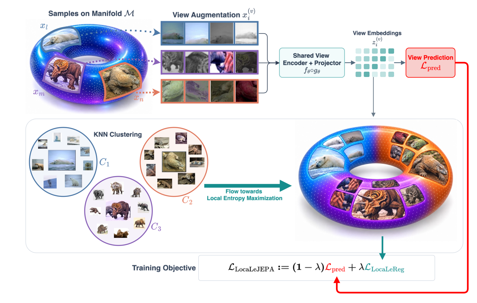
Each of N images has V augmented views. A shared encoder and projector produce (z_i^{(v)}\in\mathbb R^d). Their per-image mean is
This term encourages the views of the same image to agree. The local regulariser addresses the distribution of embeddings across images. Combining them gives
Keep the encoder representation and the projected training embedding separate. In the shared experimental interface, frozen downstream readouts use 512-dimensional encoder representations. The smaller backbones use a 2048–2048–16 projector for regularisation; ViT-L/14 uses the 2048–2048–512 projector from LeJEPA’s large-model settings. A 16-dimensional regularisation space does not mean the downstream classifier receives only 16 features.
The hyperbolic and equivariant encoders also feed the common Euclidean projector. The experiments therefore test compatibility with those encoder priors; the implementation is not computing exact geodesic neighbourhoods and intrinsic heat kernels in every backbone’s output geometry.
Neighbourhoods are shared across views
For each image, compute its view-mean embedding. Run cosine-similarity k-means, using at most ten iterations, on detached copies of those means. The resulting image-index partition (C_1,\ldots,C_K) is shared by all views: different augmentations of the same image remain in the same neighbourhood for the distribution tests.
The assignment step is not differentiated. Once assignments are fixed, however, gradients flow through the projected features and through their per-view cluster means. Detaching the clustering decision is different from detaching the whole local objective.
Clusters containing fewer than four images are excluded from the regulariser. If none survive, the method falls back to the same centred uniform-ball test on the complete batch, separately for each view. These images still participate in view prediction; exclusion concerns an unreliable small-sample distribution test.
The threshold of four is a practical heuristic. It is neither a proof that four examples identify a distribution nor a requirement for the discrepancy to exist mathematically. Appendix A.2 explicitly investigates the finite-sample limitations.
Centre each neighbourhood without moving all centres together
For a retained cluster q and view v, form
It is the distribution of residuals r that is matched to the target. Entropy is translation-invariant, so this removes an unnecessary preference for one absolute cluster location.
An illustrative one-dimensional example makes the effect visible. Consider two fixed neighbourhoods ({9,10,11}) and ({-11,-10,-9}). Their means are 10 and −10, but both produce residuals ({-1,0,1}). The local shape test sees the same spread in both and does not directly demand that the two means coincide. This example illustrates translation invariance; those three residuals are not an exact sample-level match to the training target, and the actual minimum accepted size is four.
Location is free conditional on the neighbourhood partition. Moving features can change future cosine-based assignments, and the shared network and agreement loss still couple the training problem. Local centring therefore does not make all clusters independent optimisation problems or explicitly push their means apart.
Why the target is a ball—and why its radius matters
The reference is uniform over the interior of a d-dimensional Euclidean ball, rather than on its boundary sphere. For (Y\sim\operatorname{Unif}(B_R^d)), symmetry gives
Choosing (R=\sqrt{d+2}) makes that covariance identity, matching the scale of SIGReg’s standard Gaussian. At d=16, the radius is (\sqrt{18}). The change is therefore not merely shrinking the embeddings to a smaller variance: the distributions have matched covariance but different support and higher-order structure.
Uniform in a ball also does not mean uniform along every one-dimensional projection. A projected marginal has density proportional to ((1-s^2/R^2)^{(d-1)/2}) inside its support. Replacing it with a scalar uniform target would implement a different regulariser.
Appendix A.3 explains how another radius can be related by rescaling. That equivalence requires adjusting both the characteristic-function frequencies and the prediction-loss scale. Changing only the radius while leaving the remaining computation untouched changes the effective objective.
Compare distributions through random projections
Rather than estimate a full d-dimensional density, LocaLeReg tests random one-dimensional projections. For unit direction u, the empirical characteristic function of a cluster’s residuals is
A characteristic function records distributional information through averaged complex oscillations. The uniform-ball reference has an analytic, rotationally symmetric counterpart:
Here (J_{d/2}) is the Bessel function of the first kind. The reference can be precomputed for a fixed dimension and frequency grid. The removable singularity at zero must be handled using its limit.
The sliced Epps–Pulley discrepancy is
The Cramér–Wold principle motivates checking projections: agreement in every direction determines a multivariate distribution. A finite set of directions and frequencies is an approximation, not that infinite guarantee. The smaller-model implementation uses 256 directions and trapezoidal integration over [−3,3], exploiting symmetry with 17 nonnegative frequencies. ViT-L/14 uses 1,024 directions and [−5,5].
K changes locality, sample support and loss scale
Increasing K makes neighbourhoods finer, but also leaves fewer observations in each test. At roughly balanced size N/K, the sample-count factor inside each discrepancy makes the regulariser scale approximately with N/K. Holding lambda fixed while changing K therefore does not isolate geometry alone.
This is why the paper compares K=4, lambda=0.1 with K=1, lambda=0.025: these match the nominal sample-count scaling of the regulariser. The full loss still contains its stated prediction coefficient (1-\lambda). On the three 128-pixel encoders, the matched-strength comparison retains positive gains from locality. The analogous low-weight ViT-L/14 control trains poorly, so the paper does not claim the same clean control for that model.
The relevant N is the population used for the local statistic. On ImageNet, an optimiser step spans 256 images for the smaller models, but neighbourhoods are formed independently within 64-image shards. A nominal global batch of 256 therefore does not provide 64 examples to each of four local clusters; a balanced local partition has about 16.
The appendix also shows that distinguishing covariance-matched ball and Gaussian samples becomes harder as projector dimension grows. Their one-dimensional marginals become increasingly similar. More locality is consequently a tradeoff, not a rule that larger K must improve learning.
ImageNet results: compare against the stronger baseline
All four encoder families are pretrained for 100 epochs on ImageNet-1K. Evaluation freezes the encoder and uses the final checkpoint, with a cosine-weighted k-NN readout at k=20 and a separately trained linear probe. These are representation evaluations, not full end-to-end fine-tuning results.
The table below selects the matched-settings LeJEPA baseline for the smaller encoders and the shared published ViT-L recipe for the large model. Values are percentages from Table 2 of v1; LocaLeJEPA uses K=4.
| Encoder | Linear: LeJEPA → LocaLeJEPA | k-NN: LeJEPA → LocaLeJEPA | Seven-dataset transfer mean |
|---|---|---|---|
| Euclidean ViT-S/8 | 51.6 ± 0.28 → 62.1 ± 0.27 | 38.9 ± 0.09 → 50.1 ± 0.12 | 64.3 ± 0.13 → 72.3 ± 0.29 |
| Hyperbolic ViT-S/8 | 51.6 → 61.9 | 39.4 → 50.6 | 64.1 → 72.1 |
| D4-equivariant ResNet-50 | 48.8 → 55.2 | 39.7 → 47.5 | 58.8 → 63.0 |
| Euclidean ViT-L/14 | 54.7 → 61.0 | 46.0 → 47.4 | 61.3 → 65.5 |
The plain ViT-S/8 values summarise three pretraining seeds; the other rows are single pretraining runs. All use one linear-probe seed. The smaller encoders use 128-pixel inputs and the large encoder 238-pixel inputs, so comparisons should be made within each row, not interpreted as a controlled ranking of backbone sizes.
Matching settings matters. For the plain ViT-S/8, changing LeJEPA’s optimisation settings already raises linear top-1 from 44.6 to 51.6. The further improvement to 62.1 is the comparison relevant to the new objective under that stronger baseline.
Transfer uses DTD, FGVC-Aircraft, CIFAR-10, CIFAR-100, Flowers-102, Food-101 and Oxford-IIIT Pets. Each frozen encoder receives a task-specific linear classifier, with learning-rate selection on a training holdout. K=4 improves all seven reported datasets over the relevant LeJEPA baselines. The reported average weights datasets equally rather than weighting by their number of test images.
Which part of the change earns the improvement?
A single-neighbourhood version already improves the smaller backbones. K=1 is a global centred ball target, so that result cannot be attributed to multiple local neighbourhoods. Moving to K=4 adds a further gain, and the matched-strength controls help separate locality from the sample-count scaling described above.
Another control keeps the same local partition but applies Gaussian matching to uncentred cluster embeddings. This LocaLeJEPA-SIGReg variant falls below the matched-settings LeJEPA baseline on the reported hyperbolic and equivariant encoders. Merely partitioning the batch is therefore insufficient to explain the gains.
That control changes both centring and reference distribution. It supports the combined centred local target, but does not separately identify how much of the gain belongs to centring alone versus the ball distribution alone. Keeping that distinction explicit makes the evidence more useful for the next experiment.
The dynamic schedule starts at K=1 and progressively adds neighbourhoods. It performs similarly to fixed K=4 on the reported hyperbolic and equivariant ImageNet settings. This supports a practical alternative for introducing locality; it does not establish that the schedule follows an exact heat flow or is universally optimal.
Does useful geometry survive beyond classification?
A rotating COIL-100 object provides a known circular structure. The paper compares PCA views with persistent-homology measurements, using the latter to examine loops beyond what a two-dimensional plot alone can establish. The results are evidence about these controlled representations, rather than a blanket guarantee of topology preservation on arbitrary data.
The two-figurine experiment asks a stronger transfer question. Encoders are pretrained on Imagenette and then frozen. A separate dataset varies two rotation angles independently, so its underlying parameter space is (S^1\times S^1), a torus. Readouts predict the angles from the frozen features.
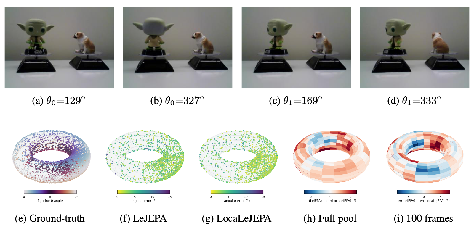
With the full labelled probe pool, Table 1 reports wrapped angular MAE of 3.30 ± 0.05° for SIGReg and 2.67 ± 0.05° for LocaLeJEPA with K=2. With 100 labelled training frames, the comparison is 11.0 ± 0.4° versus 9.0 ± 0.3°. The standard deviations vary the probe split, not the pretraining seed. These encoders use the study’s Imagenette pretraining and checkpoint-selection protocol, distinct from the final-checkpoint ImageNet table.
The result connects the geometric motivation to recoverable information: a small readout can recover the underlying angles more accurately. It does not imply that every visible torus reconstruction is an isometric embedding or that classification accuracy alone measures topology.
What scalability means here
The clusters form a disjoint partition, so the distribution statistic remains linear in the total number of samples for fixed sketch and frequency settings. Clustering adds work. Appendix A.4 gives additional time (O(INKd+KdS)) and memory (O(NK+KdS)) relative to global SIGReg, with I k-means iterations and S sketch directions.
In the reported A100-40GB timing experiment, a ViT-S/8 step takes 0.263 seconds with SIGReg and 0.278 seconds with LocaLeJEPA: 5.7% additional end-to-end time for that configuration. The isolated regulariser has a much larger relative overhead, so the end-to-end figure should not be read as a universal cost ratio. K, batch size, projection dimension and backbone cost all matter.
The practical contribution is a local distribution constraint that can be implemented with batching, clustering and projected statistics. It does not require estimating a global density or recomputing the learned manifold’s exact heat kernel at every training step.
Where this fits in the JEPA book
LeJEPA explains why agreement needs a distribution constraint. LocaLeJEPA asks how that constraint should change when geometry matters. V-JEPA 2.1 studies local supervision in a different sense: dense spatial and temporal features. Here, locality concerns neighbourhoods of images in projected representation space, rather than simply smaller image patches.
The new k-means chapter supplies the clustering background, while PCA explains what the visualisations retain and discard. The paper brings these familiar tools into a new role: organising where an anti-collapse constraint acts, rather than using clustering labels as the final learning target.
Recap
- LocaLeJEPA replaces a prescribed global Gaussian cloud with centred distribution matching inside learned neighbourhoods.
- The uniform-ball target has identity covariance at radius \(\sqrt{d+2}\), so its difference from the Gaussian goes beyond scale.
- Assignments are shared across views and detached; gradients still pass through local means and residuals.
- K controls locality, sample support and regulariser scaling. Matched-strength experiments are essential to interpreting its effect.
- Frozen-feature recognition, transfer and controlled rotation recovery provide complementary evidence; they are not interchangeable claims.
- The broader lesson is to let geometry influence the anti-collapse objective, rather than treating one global reference distribution as suitable for every representation space.
References
- Tandon, K., Borgi, A., Snopov, P., García-Redondo, I., D’Ascenzo, D., Cultrera di Montesano, S., Silvestri, F., Liò, P., Dominici, F., Balestriero, R., and Battiloro, C. LocaLeJEPA: Maximum Entropy Representations under Geometric Priors. arXiv:2610.28458v1, 2026. Method: Sections 3–4 and Appendix A; experiments: Tables 1–3 and Appendices B–D.
- Authors’ LocaLeJEPA repository.
- Balestriero, R., and LeCun, Y. LeJEPA: Provable and Scalable Self-Supervised Learning Without the Heuristics. 2025. See also the LeJEPA chapter.