
Sheaf Neural Networks: A Complete Research Guide
Published:
The big idea
Do not force neighbouring nodes to be equal. Learn how they should be related, through a linear map attached to each edge.
Why it matters
That single change gives one language for heterophily, signed and directional relations, and diffusion richer than a plain graph Laplacian allows.
Where the book is
The paper chapters are live now. The foundations and theory chapters are still being written, so this overview carries the maths you need to read them.
The problem, stated precisely
A GCN layer propagates with \(\hat{A} = \tilde{D}^{-1/2}\tilde{A}\tilde{D}^{-1/2}\), which is an averaging operator. Averaging has a fixed point, and repeated averaging converges to it: features collapse towards a single degree-scaled direction. That is oversmoothing, and it is not a bug in the implementation, it is what averaging does.
It also encodes an assumption. Adding \(h_u\) to \(h_v\) only means something if the two vectors are expressed in the same basis. On a heterophilic graph, where an edge signals difference rather than similarity, that assumption is actively wrong.
The core object
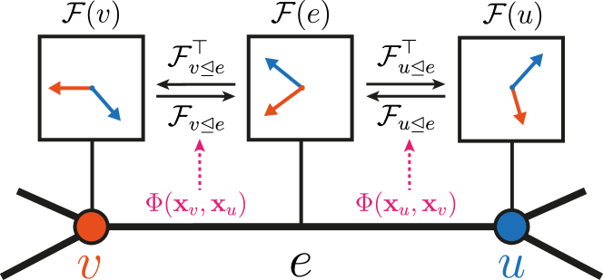
A cellular sheaf \(\mathcal{F}\) on a graph \(G = (V, E)\) assigns:
- a node stalk \(\mathcal{F}(v) \cong \mathbb{R}^{d}\) to each \(v \in V\);
- an edge stalk \(\mathcal{F}(e) \cong \mathbb{R}^{d}\) to each \(e \in E\);
- a restriction map \(\mathcal{F}_{v \trianglelefteq e} : \mathcal{F}(v) \to \mathcal{F}(e)\) for each incident pair.
The coboundary \(\delta_0\) measures disagreement across an edge, after transport:
The sheaf Laplacian is \(\Delta_{\mathcal{F}} = \delta_0^{\top}\delta_0\), a block matrix with
Because it is built as \(\delta_0^{\top}\delta_0\), it is symmetric and positive semi-definite, and its kernel is exactly the space of global sections. Set every restriction map to the identity and it collapses to the familiar case:
So the graph Laplacian is the sheaf Laplacian of the trivial sheaf. Everything a GCN does, a sheaf GNN can do by choosing identity maps, and it has \(d \times d\) more room per edge when identity is the wrong choice.
The pipeline, end to end
Definitions settle nothing until you watch a signal move through them. Here is one full step, from raw node features to a diffusion update.
Every number above is checkable. With \(\mathcal{F}_{u \trianglelefteq e} = I\) and \(\mathcal{F}_{v \trianglelefteq e} = R(90^\circ)\):
The resulting \(\Delta_{\mathcal{F}}\) has eigenvalues \(\{0, 0, 2, 2\}\), so its kernel is two-dimensional: on this graph there is a whole plane of assignments the sheaf considers globally consistent. A graph Laplacian on two connected nodes has a one-dimensional kernel, the constants. That gap is the extra room sheaf diffusion has to work in.
What changes, concretely
| Standard GCN | Sheaf GNN | |
|---|---|---|
| Operator | graph Laplacian \(L\) | sheaf Laplacian \(\Delta_{\mathcal{F}}\) |
| Edge weight | one scalar | a \(d \times d\) linear map |
| Propagation | \(H \leftarrow \hat{A}H\) | \(H \leftarrow (I - \Delta_{\mathcal{F}})H\) |
| Depth limit | collapses to a constant direction | converges to \(\ker(\Delta_{\mathcal{F}})\), which can separate classes |
| Heterophily | destructive averaging | signed or rotating maps make disagreement meaningful |
The fourth row is the theoretical heart. Oversmoothing is not avoided by making the operator weaker; it is avoided by making its null space richer. A graph Laplacian has an essentially one-dimensional-per-component null space. A sheaf Laplacian’s null space is the space of global sections, and with the right restriction maps that space is large enough to hold a separating assignment.
The whole story in one paragraph
A sheaf equips every node and edge with a vector space and every incidence with a linear map; the sheaf Laplacian then measures inconsistency after transporting signals through those maps. Accept that one formulation and a set of separately-studied GNN problems start to look like one problem: heterophily, sign structure, gauge symmetry, directional flow, and the null-space account of oversmoothing.
What is live now
The paper chapters are published; the foundations and theory chapters are still in draft. If you are arriving new, read them in this order:
Suggested reading order
- PolyNSD, replaces the fixed diffusion step with a Chebyshev polynomial in \(\Delta_{\mathcal{F}}\). The clearest entry point to what the operator actually does.
- DNSD, why sheaf diffusion stalls at depth, and what it costs to fix. Read this second: it is the sharpest critique of the framework from inside it.
- HetSheaf, sheaves on heterogeneous graphs, where node and edge types condition the restriction maps.
- SheafPool, graph-level readout that respects the sheaf's basis ambiguity.
- BrainDyn, sheaves inside a neural ODE, applied to brain dynamics. The most different thing in the book.
Still to come: the foundations run (what a sheaf is, cellular sheaves on graphs, cohomology, the Laplacian spectrum, connection Laplacians), the theory run (oversmoothing, heterophily, oversquashing, expressiveness, Hodge decomposition), and the extensions run (cosheaves, simplicial sheaves, multi-relational and temporal sheaves).
Key papers at a glance
References
- Hansen, J., & Gebhart, T. (2020). Sheaf Neural Networks. arXiv:2012.06333.
- Hansen, J., & Ghrist, R. (2019). Toward a Spectral Theory of Cellular Sheaves. Journal of Applied and Computational Topology, 3(4), 315–358.
- Bodnar, C., Di Giovanni, F., Chamberlain, B. P., Liò, P., & Bronstein, M. (2022). Neural Sheaf Diffusion: A Topological Perspective on Heterophily and Oversmoothing in GNNs. Advances in Neural Information Processing Systems 35.
- Barbero, F., Bodnar, C., de Ocáriz Borde, H. S., & Liò, P. (2022). Sheaf Attention Networks. NeurIPS 2022 Workshop on Symmetry and Geometry in Neural Representations.
- Barbero, F., Bodnar, C., de Ocáriz Borde, H. S., Bronstein, M., Veličković, P., & Liò, P. (2022). Sheaf Neural Networks with Connection Laplacians. Topological, Algebraic and Geometric Learning Workshops 2022, PMLR.
- Zaghen, O., Longa, A., Azzolin, S., Telyatnikov, L., Passerini, A., & Liò, P. (2024). Sheaf Diffusion Goes Nonlinear: Enhancing GNNs with Adaptive Sheaf Laplacians. Proceedings of the Geometry-grounded Representation Learning and Generative Modeling Workshop, ICML 2024, PMLR 251.
- Borgi, A., Silvestri, F., & Liò, P. (2025). Polynomial Neural Sheaf Diffusion: A Spectral Filtering Approach on Cellular Sheaves. arXiv:2512.00242.
- Bourgerie, R., Girdzijauskas, Š., & Fodor, V. (2026). Deep Neural Sheaf Diffusion. arXiv:2605.19021.