
ACT: Why a Robot Policy Predicts a Chunk of Actions
Published:
Tony Z. Zhao, Vikash Kumar, Sergey Levine et al.
Read the paper (PDF)
One frame does not explain a whole movement
Intuition first. Imagine inserting a battery while the other hand steadies its holder. A single image may support several reasonable next commands, depending on the demonstrator’s timing and intended approach. Predicting each action independently can lose the coordination across the movement.
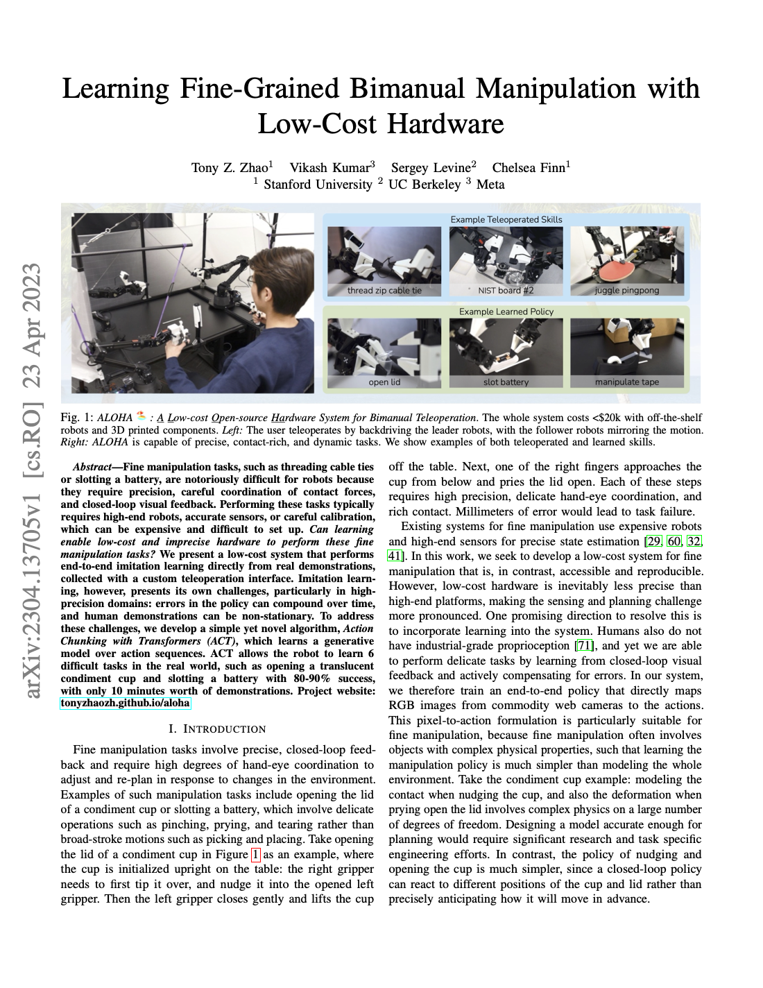
ACT maps images and joint positions to an action sequence. Its original setting uses joint-position targets for bimanual manipulation, learned from teleoperated demonstrations. The method was introduced by Zhao et al..
A sequence model with a training-time latent
Let \(o_t\) contain images and proprioception, \(q_t\) denote joint positions, and \(A_t=(a_t,\ldots,a_{t+K-1})\) be a demonstration chunk. A compact form of the training objective is
The encoder sees demonstrated future actions during training. At deployment that encoder is discarded, and the original ACT procedure sets \(z=0\), the prior mean. The policy uses current observations to predict the chunk. It does not receive future ground-truth actions at inference. The paper details this training–deployment distinction.
Two horizons that need separate names
The prediction horizon is the number of actions output by the model. The execution horizon is how many commands are applied before another policy query incorporates fresh observations.
For an illustrative 50 Hz control loop, a chunk of 20 actions describes 0.4 seconds. Executing all 20 before looking again leaves 0.4 seconds without a new policy decision. Querying every control step incorporates another observation every 0.02 seconds, if inference and sensing can meet that deadline.
Those systems use the same chunk length and have very different feedback behaviour.
Worked example: temporal ensembling
Suppose three overlapping chunks predict joint targets \(0.20\), \(0.24\), and \(0.22\) radians for the same execution time. Use illustrative normalised weights \(0.5\), \(0.3\), and \(0.2\), ordered from oldest prediction to newest:
This smooths disagreement between plans for one timestamp. Averaging \(a_t\), \(a_{t+1}\), and \(a_{t+2}\) within a single plan instead mixes commands intended for different times.
The original ACT weighting uses \(w_i=\exp(-mi)\) with index zero assigned to the oldest prediction; normalisation makes the weights sum to one. Check the indexing before interpreting the decay parameter. This detail is specified in the temporal-ensemble description.
What the model cannot fix for you
If the camera timestamp lags behind the joint observation, the model receives a physically inconsistent scene. If training actions are absolute joint targets but deployment interprets them as increments, even an accurate predictor commands the wrong movement. Verify alignment, units, action meaning, and inference latency before tuning architecture depth.
Also split demonstrations by complete episode. Randomly splitting overlapping action windows can put almost identical sequences on both sides of the evaluation boundary.
Compare this demonstration-based approach with residual RL, which learns corrections from rewards, and learned MPC, which scores future sequences through a dynamics model.
References
- Zhao, T. Z., Kumar, V., Levine, S., & Finn, C. Learning Fine-Grained Bimanual Manipulation with Low-Cost Hardware. RSS 2023.