
ONDA: Oscillatory Neural Dynamics over Sheaves
Published:
Authors: Jan-Willem Van Looy*, Alessandro Trenta*, Alessio Gravina*, Alessio Borgi*, Ferdinando Zanchetta, Pietro Liò, Davide Bacciu, Rita Fioresi. *Equal contribution.
Preprint: arXiv:2610.10018, submitted 7 October 2026 · PDF · Full text
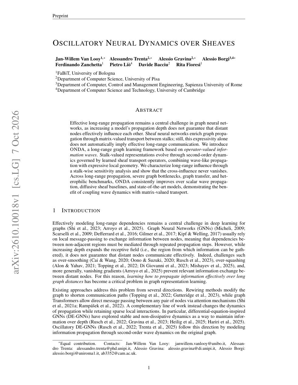
In plain words: imagine a network of connected instruments. Each connection can change the direction and mixture of a signal, while each instrument has its own ongoing vibration. ONDA learns those connections and evolves the vibrations together. The central idea is to learn both how information is transformed locally and how it stays influential as it travels.
Reaching a node is only the beginning
Stacking message-passing layers expands a GNN’s receptive field. After enough layers, a distant node can, in principle, affect the prediction. But being inside the receptive field is weaker than having a useful influence.
Repeated averaging can wash out distinctions between representations. A narrow graph bridge can force many signals through the same small channel. Gradients connecting a source node to a distant target can become tiny. These difficulties are related, but they are not identical: a graph can have a severe information bottleneck even when its diameter is small.
Sheaf neural networks improve the local interaction. Instead of weighting every neighbour’s representation by a scalar, they learn linear maps between local vector spaces. That gives the model much richer ways to transform a message. Yet a richer transformation at each edge does not, by itself, specify dynamics that preserve useful signals across many edges.
Our paper joins these two questions:
- How should a message change across an edge? Learn the transport geometry with a cellular sheaf.
- How should representations evolve over depth? Use oscillatory dynamics, with a state and a velocity.
This is ONDA: Oscillatory Neural Dynamics on Sheaves. The paper’s title uses “over sheaves”; the model name abbreviates “on sheaves”.
The sheaf is the medium through which waves travel
A cellular sheaf assigns a vector space, or stalk, to each node and edge. A node state \(X_v\) lives in its node stalk. For an edge \(e=\{u,v\}\), restriction maps
put the two endpoint states into a shared space. This lets us compare signals whose original coordinates may mean different things.
The sheaf Laplacian collects these discrepancies:
The star denotes the adjoint, which is the transpose with Euclidean inner products. First map both endpoints into the edge stalk, then compare them, and finally map the discrepancy back to the receiving node. Summing over incident edges gives the local update.
For an undirected sheaf, this construction produces a self-adjoint, positive semidefinite operator. If all stalks are one-dimensional and all restriction maps are the identity, it reduces to the usual graph Laplacian.
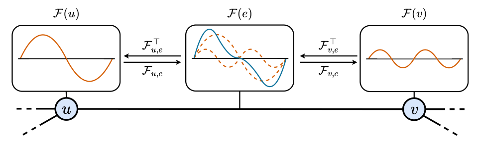
In ONDA, the learned sheaf acts as a propagation medium. Its maps determine how a wave is transformed at each interaction. Two signals can reinforce or cancel after they have been expressed in a common edge space.
This is more expressive than sending scalar-weighted copies of a signal. A matrix can change different directions differently, and its composition along a path determines the accumulated transformation.
From diffusion to a wave equation
Consider first a fixed sheaf and a single feature channel. Continuous sheaf diffusion follows
Along an eigenvector with eigenvalue \(\lambda\), the amplitude evolves as \(e^{-\lambda t}\). Positive-frequency components decay; the zero-eigenvalue component remains.
The conservative core of ONDA instead follows
Now each positive-eigenvalue mode behaves like an oscillator. With zero initial velocity, its amplitude is multiplied by \(\cos(t\sqrt{\lambda})\). It changes sign and passes through zero, but its envelope does not shrink.
| Property | Fixed-sheaf heat flow | Conservative sheaf wave |
|---|---|---|
| Evolving variables | State \(X\) | State \(X\) and velocity \(V\) |
| Equation | \(\dot X=-L_{\mathcal F}X\) | \(\ddot X=-L_{\mathcal F}X\) |
| Mode response, zero initial velocity | \(e^{-\lambda t}\) | \(\cos(t\sqrt{\lambda})\) |
| Positive-frequency behaviour | Exponential attenuation | Persistent oscillation |
| Local geometry | Learned restriction maps | Learned restriction maps |
The extra velocity provides memory of how the representation was moving. The next state depends on both the current configuration and its accumulated motion.
The learnable ONDA block
Purely conservative dynamics keep every mode active. A prediction task may need to suppress irrelevant information or introduce an additional learned drive. The full model therefore adds feature transformations, dissipation, and forcing:
Here \(X\in\mathbb R^{nd\times c}\) stacks \(n\) nodes, stalk dimension \(d\), and \(c\) feature channels.
- \(W_1\in\mathbb R^{d\times d}\) mixes coordinates inside a stalk.
- \(W_2\in\mathbb R^{c\times c}\) mixes feature channels.
- \(R_\theta(X)\geq0\) controls state-dependent dissipation.
- \(F_\theta(X)\) supplies a learned forcing term.
The sheaf term couples neighbouring nodes. Dissipation and forcing let the model adapt how much information to retain and how to drive the evolving state.
Turning the differential equation into layers
Introduce \(V=\dot X\) and a step size \(h>0\). The update first changes velocity, then advances the state using that new velocity:
One block runs several of these propagation steps and then applies an MLP. The resulting representation becomes the next block’s input, and that block initialises its velocity from its input representation. A task-specific decoder reads the final block output.
The distinction between a block and an integration step matters: several steps can evolve a representation under the same transport geometry before a nonlinear transformation changes it.
Fixed or adaptive transport
In the fixed setting, the restriction maps are inferred once from the block input and reused throughout its propagation steps. In the adaptive setting, they are recomputed from the evolving features at every step.
The paper considers diagonal, orthogonal, low-rank, and general restriction maps, along with normalised sheaf operators and a directed variant. In that directed variant, the two edge orientations can have independently learned maps and each discrepancy is applied at the receiving endpoint.
These are modelling choices with different costs and properties. In particular, the self-adjoint spectral analysis below concerns the conservative fixed-sheaf setting, rather than every possible adaptive or directed configuration.
What the theory says about long-range influence
To isolate the oscillatory mechanism, fix the sheaf inside one block, set the feature weights to the identity, and remove dissipation and forcing:
Perturb the initial state at node \(u\) while holding the initial velocity fixed. How much can that perturbation affect node \(v\)?
The answer is a matrix-valued sensitivity between their stalks:
It describes both the strength of the response and how directions in the source stalk become directions in the target stalk.
Paths explain where a signal can go
Expand the cosine operator as a power series:
Each block of \(L_{\mathcal F}^{k}\) is a sum of ordered products along length-\(k\) walks, allowing steps that remain at a node. If the shortest path from \(u\) to \(v\) has length \(r\), all terms with \(k<r\) vanish.
The geometry therefore enters twice: the graph determines the available walks, and the restriction maps determine the transformations accumulated along them. Disconnected nodes cannot influence one another. Even connected nodes can have cancellations or degenerate transport, so connectivity alone does not guarantee a nonzero response.
The spectrum explains why influence persists
For the self-adjoint sheaf Laplacian, write \(L_{\mathcal F}=\sum_\lambda\lambda P_\lambda\). Then
The zero-frequency part is constant. Every positive-frequency contribution oscillates rather than decaying exponentially.
The discrete network retains the effect under a stability condition
For the corresponding conservative discrete updates, Theorem 1 assumes
Under this condition, the source-to-target response is bounded and, if nonzero at some step, does not converge to zero as depth tends to infinity. For the symmetrically normalised sheaf Laplacian, whose spectrum lies in \([0,2]\), \(0<h<\sqrt2\) is sufficient.
Locality remains intact: a node \(r\) edges away cannot influence the target before \(r\) discrete propagation steps. ONDA changes what happens to information as it travels; it does not create shortcuts in the graph.
The theorem explains the conservative mechanism. Learned damping, forcing, nonlinear transformations, adaptive maps, and directed operators require their own consideration; the same guarantee does not automatically extend to the entire model family.
A two-node example
Take two nodes joined by an edge, with scalar stalks and identity restriction maps:
The average mode has eigenvalue \(0\), and the difference mode has eigenvalue \(2\). The receiving node therefore has state
Heat flow moves both nodes toward the same value, \(1/2\). The wave repeatedly transfers the initial signal between them: at \(t=\pi/\sqrt2\) the receiver reaches \(1\), and at \(t=2\pi/\sqrt2\) it returns to \(0\).
This example also shows why “influence never vanishes” needs care: the wave response is zero at recurring times, but it never settles into permanent attenuation. With higher-dimensional stalks, learned restriction maps also change the directions in which information arrives.
Experiments: distance and bottlenecks
The experiments separate several obstacles to communication. All numbers below are from the v1 paper.
ECHO-Synth: predictions that require distant information
ECHO-Synth tests single-source shortest paths (SSSP), node eccentricity, and graph diameter. The table below reproduces selected rows from Table 1; lower mean absolute error is better.
| Model | SSSP MAE ↓ | Eccentricity MAE ↓ | Diameter MAE ↓ |
|---|---|---|---|
| GRIT | 0.121 ± 0.013 | 5.091 ± 0.158 | 1.014 ± 0.046 |
| SONAR | 0.527 ± 0.254 | 2.393 ± 0.808 | 1.239 ± 0.151 |
| NSD | 0.231 ± 0.038 | 4.672 ± 0.315 | 1.448 ± 0.097 |
| CSNN | 0.421 ± 0.165 | 4.522 ± 0.048 | 1.134 ± 0.094 |
| ONDA | 0.085 ± 0.019 | 0.885 ± 0.158 | 1.183 ± 0.020 |
ONDA has the lowest reported error on SSSP and eccentricity. It improves on both its oscillatory comparator, SONAR, and standard sheaf diffusion, NSD. Diameter prediction is more mixed: ONDA is competitive, but GRIT and several other baselines achieve lower error.
Barbell graphs: a short path can still be a hard bottleneck
The Barbell task joins two cliques with one bridge. Every node must predict the empirical feature mean of the opposite clique. The diameter is only three, but all cross-clique information must pass through the same edge.
That makes the task a useful complement to long-distance tests. It measures whether the model can collect and transmit a statistic through a narrow communication channel.
The following values convert Table 2’s \(\times10^{-3}\) units into ordinary MSE. \(N\) is the number of nodes in each clique; the graph has \(2N\) nodes. Results are means ± standard deviations over five seeds.
| Model | N = 10 MSE ↓ | N = 20 MSE ↓ | N = 50 MSE ↓ |
|---|---|---|---|
| GAT | 0.0079 ± 0.0021 | 0.4870 ± 0.3422 | 0.8520 ± 0.0290 |
| SONAR | 0.4628 ± 0.2503 | 0.7175 ± 0.2496 | 0.8090 ± 0.0680 |
| NSD | 0.9372 ± 0.0114 | 1.0051 ± 0.0078 | 0.8250 ± 0.0320 |
| CSNN | 0.4739 ± 0.1062 | 0.8908 ± 0.2654 | 0.7420 ± 0.1680 |
| ONDA | 0.0007 ± 0.0003 | 0.0009 ± 0.0005 | 0.0830 ± 0.0850 |
Under the benchmark’s convention, MSE below \(0.25\) counts as solving the task. ONDA is the only model family in the main comparison to meet that criterion at \(N=50\). Its standard deviation there also matters: the mean is strong, but performance varies across seeds.
The restriction-map ablation adds a useful detail. More expressive maps are not automatically better: diagonal ONDA gives the lowest mean error at \(N=20\) and \(N=50\) among the tested parametrisations. The gain comes from the interaction between transport and dynamics, rather than simply using the largest matrix family.
Graph transfer: carrying information up to 50 hops
In this task, source and target nodes start at \(1\) and \(0\). The model must swap their values while preserving the other node features. The paper tests line, ring, and crossed-ring graphs at distances of 3, 5, 10, and 50 hops.
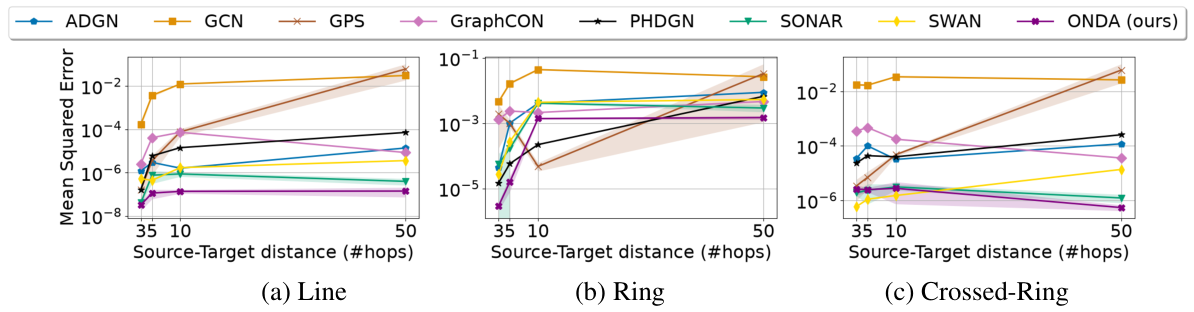
This comparison tests the combination directly: ONDA outperforms oscillatory graph baselines without sheaf transport and maintains effective transfer as the source moves farther away. It still uses local propagation throughout.
Heterophily: useful beyond explicit transfer tasks
Appendix C.2 evaluates Roman-empire, Amazon-ratings, Minesweeper, Tolokers, and Questions. ONDA improves on SONAR and NSD on all five datasets, and the paper reports third overall by average rank.
It does not lead every dataset. For example, ONDA reaches \(91.86\pm0.31\) accuracy on Roman-empire, compared with CSNN’s \(92.63\pm0.50\). These results support broader usefulness while leaving room for models designed around other inductive biases.
Cost and practical choices
ONDA keeps graph-local computation. For fixed stalk and channel dimensions, its cost scales linearly with the number of nodes and edges. It does not need dense all-pairs attention.
The extra work is still real: every node stores a velocity as well as a state, and each propagation step applies sheaf transport. General restriction maps cost quadratically in stalk dimension, whereas diagonal maps make that part cheaper. Reusing maps within a block also avoids paying the map learner’s cost at every inner step.
Training must backpropagate through the unrolled dynamics, so increasing the number of blocks or propagation steps increases activation memory unless checkpointing is used. The sparse graph scaling should therefore be read together with the chosen width, map family, and propagation depth.
Where ONDA fits in the sheaf story
Neural Sheaf Diffusion learns a geometry for diffusion. PolyNSD makes spectral filtering on that geometry more flexible. Topological Attention investigates the role of matrix-valued transport in attention.
ONDA concentrates on the evolution of information through that geometry. Its contribution is the coupling of learned sheaf transport with oscillatory dynamics, together with a stalk-wise sensitivity analysis and experiments that stress both distance and bottlenecks.
Key takeaways
- Local geometry and propagation dynamics solve different problems. Restriction maps transform messages; wave dynamics determine how those transformed signals evolve.
- A state and a velocity make depth behave differently. In the conservative setting, positive-frequency components oscillate instead of decaying exponentially.
- The guarantee has explicit assumptions. A nontrivial response persists under the fixed, conservative, self-adjoint model and a suitable discrete step size; instantaneous cancellation remains possible.
- The strongest evidence comes from communication tasks. ONDA leads SSSP and eccentricity on ECHO-Synth and handles the severe Barbell bottleneck, while remaining competitive on heterophily.
Paper and citation
This explainer follows Oscillatory Neural Dynamics over Sheaves, arXiv:2610.10018v1. Figures 1 and 2 and the first-page preview are reproduced from the paper, available under CC BY 4.0. The two-node example is an illustrative calculation of the conservative equations.
@misc{vanlooy2026oscillatoryneuraldynamicssheaves,
  title         = {Oscillatory Neural Dynamics over Sheaves},
  author        = {Jan-Willem Van Looy and Alessandro Trenta and
                   Alessio Gravina and Alessio Borgi and
                   Ferdinando Zanchetta and Pietro Liò and
                   Davide Bacciu and Rita Fioresi},
  year          = {2026},
  eprint        = {2610.10018},
  archivePrefix = {arXiv},
  primaryClass  = {cs.LG},
  url           = {https://arxiv.org/abs/2610.10018}
}