
Generalised Advantage Estimation: How Much Future Should an Update Trust?
Published:
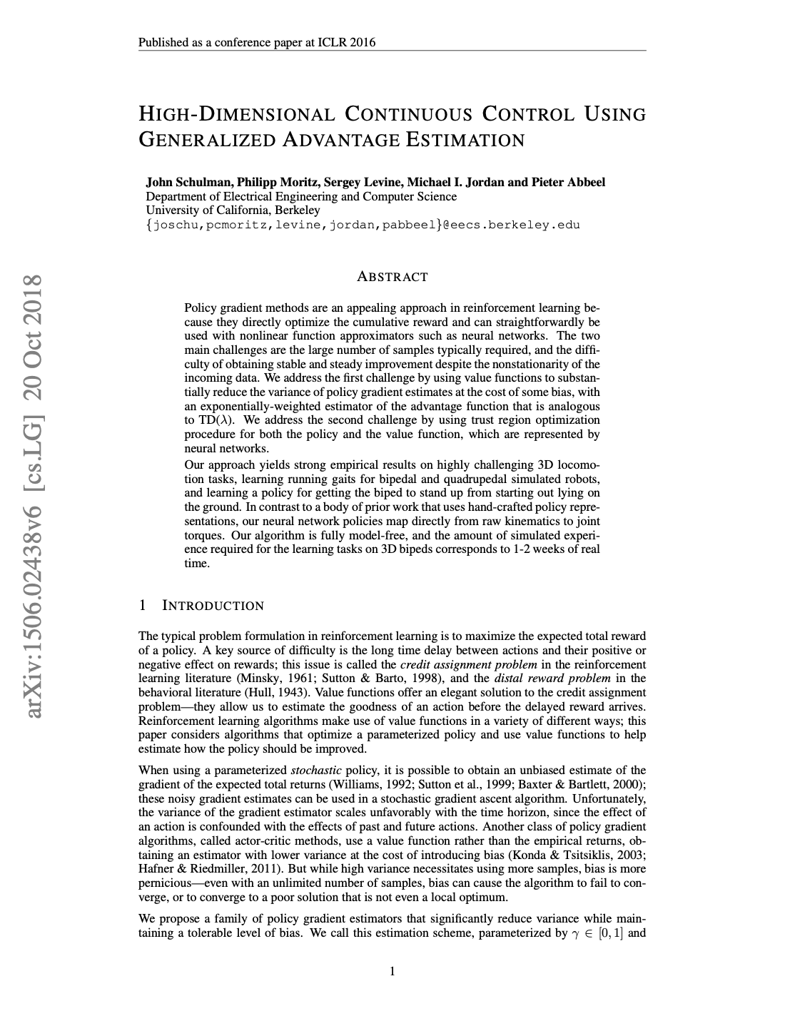
John Schulman, Philipp Moritz, Sergey Levine et al.
Read the paper (PDF)
Better than what?
Intuition first. Imagine two decisions in a game. One earns five points from an easy position where ten were expected. The other earns two points from a difficult position where zero were expected. Reward alone favours the first. Improvement over the policy’s usual outcome favours the second.
For a policy \(\pi\), the value \(V^\pi(s)\) is its expected discounted return from state \(s\). The action value \(Q^\pi(s,a)\) fixes the first action, then follows that policy. Their difference is the advantage:
Positive advantage gives an actor a reason to increase an action’s probability. The challenge is that neither true value is available during training.
From one-step errors to a longer view
Let \(V\) be the learned critic, \(r_t\) the reward following action \(a_t\), and \(\gamma\) the discount. For a rollout ending at index \(T\), GAE uses
At a true terminal state set the next-state value to zero. At a collection cutoff in a continuing episode, retain the bootstrap value. The estimator and its bias–variance analysis come from Schulman et al..
With \(\lambda=0\), only the first TD error contributes. With \(\lambda=1\), the value terms telescope into the discounted reward sum plus a boundary bootstrap, minus \(V(s_t)\). Intermediate values blend those horizons. An inaccurate critic can introduce bias when \(\lambda<1\); longer horizons typically introduce more sampling variability.
Worked example: three rewards, one backwards pass
Consider a deliberately small episode with rewards \([1,0,2]\), values \([1.5,1.0,0.5,0]\), and \(\gamma=0.9\). The final state is terminal. The TD errors are
Choose \(\lambda=0.8\), so \(\gamma\lambda=0.72\). Compute backwards:
| Step | Calculation | Advantage |
|---|---|---|
| 2 | \(1.5\) | \(1.5\) |
| 1 | \(-0.55+0.72(1.5)\) | \(0.53\) |
| 0 | \(0.4+0.72(0.53)\) | \(0.7816\) |
The middle action has a negative immediate TD error but a positive GAE estimate: the later reward changes its assessment. This is a numerical illustration, not an experimental result.
Two boundaries, two different decisions
A useful implementation keeps bootstrapping separate from continuing the trace. A true terminal transition does neither. A time-limit cutoff of an otherwise continuing task can bootstrap from its final observation, but must not carry a trace into the reset episode. A finite-horizon task whose horizon is genuinely part of the objective is different: its endpoint is terminal.
This plain Python version assumes one stored rollout, with next_values evaluated on the actual next observations before any reset:
def gae(rewards, values, next_values, terminated, episode_end,
        gamma=0.99, lam=0.95):
    advantages = [0.0] * len(rewards)
    trace = 0.0
    for t in reversed(range(len(rewards))):
        bootstrap = 0.0 if terminated[t] else next_values[t]
        delta = rewards[t] + gamma * bootstrap - values[t]
        continuation = 0.0 if episode_end[t] else trace
        trace = delta + gamma * lam * continuation
        advantages[t] = trace
    return advantages
The initial zero trace also stops accumulation at the end of the stored rollout. Its final TD error still bootstraps when appropriate. episode_end must include both termination and truncation boundaries.
What to inspect when learning stalls
Inspect advantage statistics before normalisation, critic errors, and how often rollouts end. A sign error can reward the wrong actions; a reset observation used as a bootstrap can join unrelated episodes. Increasing \(\lambda\) cannot repair either bug.
For a complementary approach to critic error in continuous control, continue with TD3.
References
- Schulman, J., Moritz, P., Levine, S., Jordan, M. I., & Abbeel, P. High-Dimensional Continuous Control Using Generalized Advantage Estimation. ICLR 2016.