
Learned Model Predictive Control: Plan with a Model, Correct with Reality
Published:
Kurtland Chua, Roberto Calandra, Rowan McAllister et al.
Read the paper (PDF)
Learning what happens next
Intuition first. To push a block onto a target, a robot can predict where several candidate pushes would move it, choose a promising one, and check the actual result. It does not have to learn a direct mapping from every possible scene to the best command.
Assume an observed state \(s_t\) sufficient for prediction. A learned dynamics model might predict a state increment,
For a horizon \(H\), stage cost \(c\), and terminal cost \(c_H\), planning chooses
Execute only \(a_0^*\). At the next step replace the predicted state with the observation and solve again. The horizon moves forward with the robot.
Worked example: replanning corrects a wrong gain
Take a one-dimensional system \(x_{t+1}=x_t+b a_t\), start at \(x_0=0\), and target \(x=1\). Suppose the model assumes \(b=1\), whereas the real gain is \(0.8\). Bound each action to \([-0.6,0.6]\).
A candidate two-step plan \([0.5,0.5]\) predicts arrival at the target. Executing it open-loop actually gives
Instead, execute the first \(0.5\) and observe \(x_1=0.4\). Even without updating the incorrect model, a new candidate command \(0.6\) now predicts reaching the target in one step. Reality gives \(x_2=0.4+0.8(0.6)=0.88\).
This particular correction reduces the error from \(0.20\) to \(0.12\). It does not eliminate it. The example compares illustrative candidate sequences, not solutions to an unspecified cost function.
What PETS adds
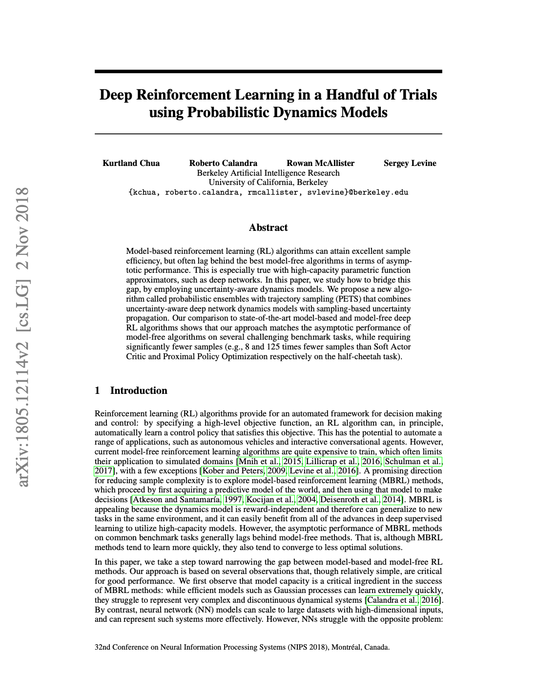
PETS trains an ensemble of probabilistic neural dynamics models. Within-model predictive variation represents transition noise; disagreement across models provides an approximation to uncertainty from limited data. Candidate action sequences are evaluated with sampled particles propagated through these models. A sampling optimiser, such as the cross-entropy method, searches the sequence space. Chua et al.
In cross-entropy optimisation, sample sequences, score them, keep an elite subset, and refit the sampling distribution. Repeat within the computation budget. This searches over future actions; it does not require fitting an actor network.
| Uncertainty | Example | What additional data can do |
|---|---|---|
| Aleatoric | Similar pushes produce variable displacement | Characterise the variability |
| Epistemic | The dataset contains few pushes at this speed | Reduce uncertainty in the fitted model |
These labels describe an intended decomposition. An ensemble is an approximation, and shared modelling assumptions can make all members confidently wrong.
Expected cost is not a safety guarantee
Imagine a candidate with a 95% chance of cost zero and a 5% chance of cost 100. Its expected cost is five. A second candidate always costs six. An expected-cost planner prefers the first, even if its rare outcome represents an unacceptable collision.
If that distinction matters, the optimisation problem needs suitable constraints or a risk-sensitive objective. Neither an ensemble nor frequent replanning automatically supplies one. This follows directly from what the objective averages.
Match prediction tests to the planner
Inspect multi-step rollouts under candidate actions, not only one-step prediction error on logged data. The optimiser may discover sequences where model errors compound. Measure planning latency too: a mathematically better plan that misses the control deadline uses stale information.
ACT also predicts action sequences, but learns them directly from demonstrations rather than scoring them through a dynamics model. Rapid motor adaptation instead uses recent interaction to condition a learned control policy.
References
- Chua, K., Calandra, R., McAllister, R., & Levine, S. Deep Reinforcement Learning in a Handful of Trials using Probabilistic Dynamics Models. NeurIPS 2018.