
Policy Gradient Methods: REINFORCE and Beyond
Published:
Why Direct Policy Optimisation?
Value-based methods such as Q-learning learn a value function and extract a policy greedily. This works well for discrete action spaces but breaks down in continuous or high-dimensional settings where the argmax over actions is intractable. Policy gradient methods sidestep this by parameterising the policy directly as \(\pi_\theta(a \mid s)\) and updating \(\theta\) to maximise expected return.
The objective is:
where \(d^\pi\) is the stationary state distribution under policy \(\pi_\theta\). We want \(\nabla_\theta J(\theta)\).
The Policy Gradient Theorem
The policy gradient theorem (Sutton et al. 1999) provides a clean expression for \(\nabla_\theta J(\theta)\) that does not require the gradient of the state distribution:
The term \(\nabla_\theta \log \pi_\theta(a \mid s)\) is called the score function or likelihood-ratio gradient. It tells us: for each action taken, push the policy parameters in the direction that makes that action more probable, scaled by how good that action was.
REINFORCE: Monte Carlo Policy Gradient
Williams (1992) proposed REINFORCE, which substitutes the full return \(G_t = \sum_{k=t}^{T} \gamma^{k-t} r_k\) for the unknown \(Q^\pi(s_t, a_t)\):
The algorithm is straightforward: roll out complete episodes, compute returns, and perform a gradient step. The estimator is unbiased — in expectation it recovers the true gradient — but the variance can be very large because \(G_t\) fluctuates enormously across trajectories.
Baselines and Variance Reduction
A baseline \(b(s)\) subtracted from the return does not change the expected gradient (since \(E[\nabla_\theta \log \pi_\theta \cdot b] = 0\)) but can substantially reduce variance:
The optimal baseline in terms of variance minimisation is proportional to the squared gradient norm, but in practice the state-value function \(V^\pi(s)\) works very well. The quantity \(A(s,a) = Q(s,a) - V(s)\) is the advantage function: it measures how much better action \(a\) is compared to the average action in state \(s\).
Using the advantage as the weight yields the advantage actor-critic family of methods.
Practical Considerations
Several implementation choices matter in practice:
- Episode length vs. batch size: REINFORCE requires full episodes; with longer horizons, variance compounds. Mini-batch updates with multiple parallel rollouts help.
- Reward normalisation: standardising returns to zero mean and unit variance per batch stabilises learning.
- Entropy regularisation: adding an entropy bonus \(H[\pi_\theta(\cdot \mid s)]\) encourages exploration and prevents premature convergence.
- Learning rate sensitivity: policy gradient methods are notoriously sensitive to step size, motivating trust-region and proximal methods covered in later posts.
From REINFORCE to Modern Policy Gradients
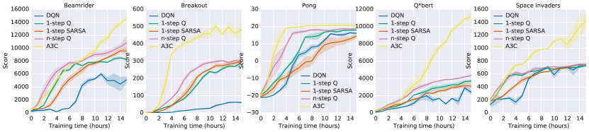
REINFORCE is the conceptual root of a large family: A3C and A2C introduce bootstrapped advantage estimates, PPO adds a clipped surrogate objective for more stable updates, TRPO enforces a hard KL constraint, and SAC incorporates maximum-entropy regularisation. Each successor addresses one limitation of vanilla REINFORCE while preserving the core log-gradient insight.
References
- Williams, R.J. (1992). Simple Statistical Gradient-Following Algorithms for Connectionist Reinforcement Learning. Machine Learning, 8(3-4), 229–256.
- Sutton, R.S., McAllester, D., Singh, S., & Mansour, Y. (1999). Policy Gradient Methods for Reinforcement Learning with Function Approximation. NeurIPS.
- Sutton, R.S., & Barto, A.G. (2018). Reinforcement Learning: An Introduction (2nd ed.). MIT Press. Chapter 13.
- Schulman, J., Moritz, P., Levine, S., Jordan, M., & Abbeel, P. (2016). High-Dimensional Continuous Control Using Generalized Advantage Estimation. ICLR. arXiv:1506.02438.