
V-JEPA 2.1: Why Dense Features Need Local Supervision
Published:
Lorenzo Mur-Labadia, Matthew Muckley, Amir Bar et al.
Read the paper (PDF)
Global understanding can coexist with poor local features
Intuition first. A model may recognise “someone is cooking” while representing the handle of a pan poorly. Classification can succeed with aggregated evidence. Grasping that handle, estimating its depth, or assigning each pixel a class requires more local information.
Mur-Labadia et al. investigate this gap in V-JEPA features. Their hypothesis is that visible context tokens can become global information aggregators when the loss directly supervises only masked positions. V-JEPA 2.1 adds supervision at the context positions and at multiple representation levels.
Make the visible positions accountable
Let \(M\) and \(C\) denote masked and visible token indices, and let \(e_i=\|\hat z_i-\operatorname{sg}(z_i)\|_1\). At one supervised level, the objective has the form
The context weights emphasise positions near a masked region. The paper uses an inverse-square-root distance weighting, together with its training schedule. The full method applies losses at multiple encoder levels and uses separate image and video patch tokenisers feeding a shared encoder. Method, official code and models.
Worked example: distance changes a token’s weight
Use the paper’s weighting shape with an illustrative base coefficient \(\lambda=0.2\). A context token one block from its closest masked token receives weight \(0.2\); a token four blocks away receives weight \(0.1\):
If both have feature error \(0.5\), their weighted contributions before averaging are \(0.10\) and \(0.05\). For a context set containing just these two tokens, the context loss is \(0.075\).
The nearer position receives stronger local consistency pressure. These numbers illustrate weighting, not the coefficients of every released checkpoint. Masked positions use their separate loss term; substituting distance zero into the context expression would misuse the formula.
Why multiple depths are useful
A transformer can change what its tokens represent from layer to layer. Supervising several depths supplies direct training signals before the final output. The paper evaluates this together with context supervision rather than assuming that a final-layer objective gives every intermediate representation the same properties.
For an independent diagnostic, freeze the backbone and train the same small segmentation head on features from different depths. Hold resolution, labels, optimisation, and evaluation split fixed. This asks where local information is accessible, rather than whether a large task-specific decoder can compensate for weak features.
Read visualisations beside quantitative evidence
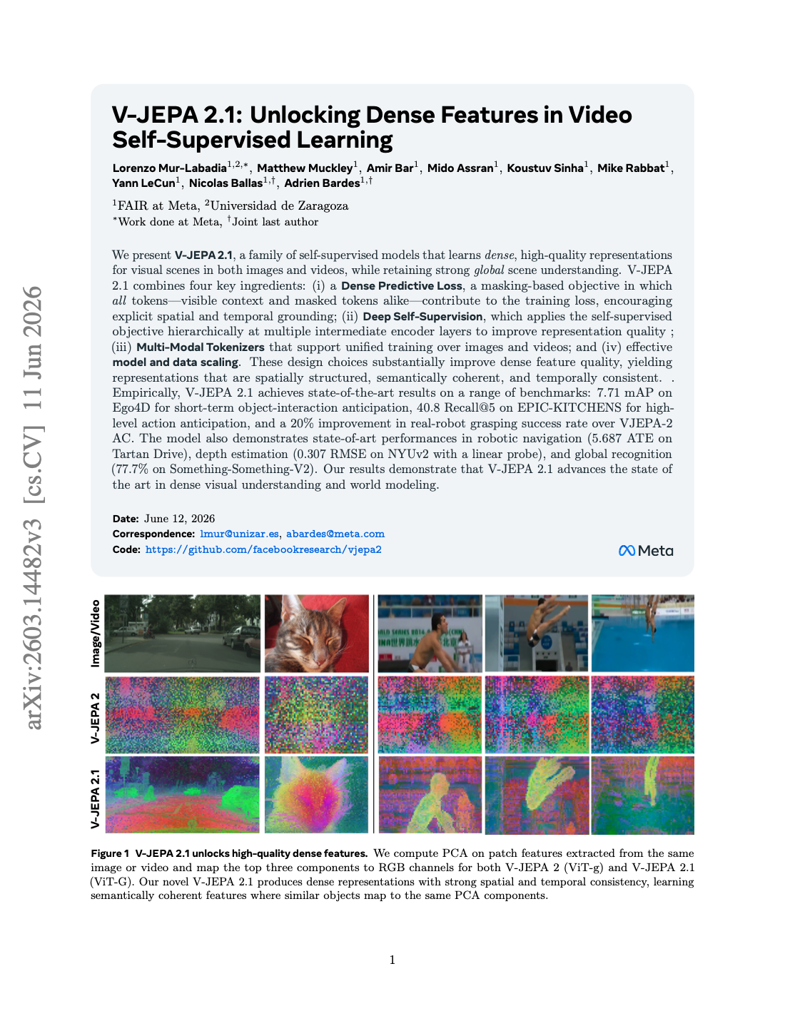
Colouring the leading principal components of a feature map can expose coherent regions. But a smooth colour map does not establish correct boundaries or calibrated depth. Compare task metrics, probe capacity, and failure cases as well as pictures.
Read V-JEPA 2 for the preceding world-model pipeline and V-JEPA for the original masked-video objective.
References
- Mur-Labadia, L., et al. V-JEPA 2.1: Unlocking Dense Features in Video Self-Supervised Learning. 2026.
- Meta FAIR. V-JEPA 2.1 code and models in the V-JEPA 2 repository.