
LeJEPA: Prediction Needs a Non-Collapsing Representation
Published:
Randall Balestriero and Yann LeCun
Read the paper (PDF)
Agreement has a trivial solution
Intuition first. Ask a model to give two photographs of the same object similar representations. Returning the same vector for every photograph satisfies the instruction. The loss needs a second requirement that distinguishes useful agreement from this shortcut.
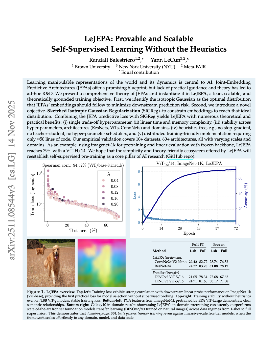
Balestriero and LeCun propose LeJEPA, pairing prediction with a regulariser that pushes embeddings towards an isotropic Gaussian distribution. Their formulation trains without the moving-average teacher or stop-gradient used in several earlier JEPA recipes.
Two terms with different jobs
In the paper’s image-view formulation, let \(z_{n,v}\) be the embedding of view \(v\) of sample \(n\), and \(\bar z_n\) the mean embedding of its global views. A compact expression is
Here \(d\) is feature dimension; SIGReg is evaluated across samples for each view and then averaged. The centre remains part of the differentiable computation. See the method and implementation and official repository.
Prediction ties together related observations. Regularisation constrains the population of representations. Neither role can be inferred from the other term’s scalar value.
How random projections reveal a collapsed cloud
SIGReg compares projected embedding distributions to a standard Gaussian using characteristic functions. For a unit direction \(u\) and projected samples \(s_n=u^\top z_n\), the empirical characteristic function is
The method aggregates discrepancies over frequencies and sampled directions. This checks more than means and variances; the paper supplies the statistical construction and its assumptions. SIGReg derivation.
Worked example: the zero embedding
If every embedding is zero, every projection is zero. Hence \(\hat\varphi_u(t)=1\) for every direction and frequency. At \(t=1\), the target value is \(e^{-1/2}\approx0.6065\). The squared discrepancy at that single frequency is
The prediction term may be zero while this distribution discrepancy is positive. This calculation illustrates the mechanism; it is not the complete SIGReg loss, which aggregates and weights its comparisons.
Now consider embeddings drawn independently of their images from a Gaussian. They could have an excellent marginal distribution but would not consistently agree across related views. A useful representation must satisfy both requirements while preserving information relevant to downstream tasks.
What the theory does and does not establish
Read the optimality result together with its task family, probe, distributional assumptions, and constraints. A theorem about favourable feature geometry does not show that an arbitrary optimiser will discover the right visual concepts on an arbitrary dataset.
For practical evaluation, keep the encoder fixed and compare task heads under the same data split. Also inspect feature variance and covariance, and test whether changes that matter to the task remain distinguishable. These diagnostics answer different questions and should not be compressed into one “healthy representation” score.
Compare the target-encoder approach in I-JEPA and the contrastive training used by VL-JEPA.
References
- Balestriero, R., & LeCun, Y. LeJEPA: Provable and Scalable Self-Supervised Learning Without the Heuristics. 2025.
- Authors’ LeJEPA implementation.