
Message Passing: The Universal GNN Framework
Published:
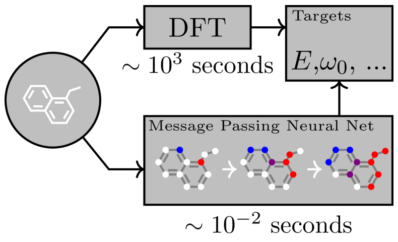
The Framework
The MPNN framework (Gilmer et al., 2017, ICML) defines GNN computation through a series of message passing steps. At each step \(t\):
Where:
- \(h_v^{(t)} \in \mathbb{R}^{d_t}\), the representation of node \(v\) after \(t\) message passing steps; \(h_v^{(0)}\) is the input feature vector.
- \(\mathcal{N}(v)\), the set of neighbours of \(v\) in the graph.
- \(e_{uv}\), the (optional) feature vector of the edge between \(u\) and \(v\).
- \(m_v^{(t+1)}\), the aggregated message arriving at \(v\) at step \(t+1\).
- \(\operatorname{MSG}\), the message function, computing what a neighbour sends.
- \(\operatorname{AGGREGATE}\), combines all incoming messages (must be permutation-invariant, since \(\{\cdot\}\) is a multiset, not an ordered list).
- \(\operatorname{UPDATE}\), computes the new representation from the old one plus the aggregated message.
Concrete Worked Example: One Full MPNN Step
Let node \(B\) have features \(h_B = [1, 0]\), with three neighbours \(\mathcal{N}(B) = \{A, C, D\}\) whose features are \(h_A = [0, 1]\), \(h_C = [1, 1]\) and \(h_D = [0, 0]\).
Step 1, Compute messages (using the identity message function, \(\operatorname{MSG}(h_v, h_u, e_{uv}) = h_u\), i.e. just pass the neighbour’s features along):
Step 2, Aggregate (sum):
Step 3, Update (concatenate own features with the aggregate, apply a learned linear map \(W \in \mathbb{R}^{2 \times 4}\) and a ReLU):
Here \(\Vert\) denotes concatenation, so \([\, h_B \Vert m_B \,] \in \mathbb{R}^4\). After this one layer, \(B\)’s new 2-dimensional embedding encodes information from all three of its neighbours.
Step 1: Message Function
The message function computes what each neighbour sends. The simplest choice: just send the neighbour’s features.
Here \(W\) is a learned weight matrix shared by all edges, and \(\alpha_{vu}\) is the scalar attention weight GAT places on the edge \(u \to v\). Including edge features \(e_{uv}\) allows the model to distinguish bond types in a molecule or relationship types in a knowledge graph.
Step 2: Aggregate Function
The aggregation combines all messages. It must be permutation-invariant (the order of neighbours shouldn’t matter):
| Aggregator | Formula | Properties |
|---|---|---|
| Sum | \(\sum_{u \in \mathcal{N}(v)} m_{u \to v}\) | Keeps the size of the neighbourhood |
| Mean | \(\frac{1}{\lvert \mathcal{N}(v) \rvert} \sum_{u \in \mathcal{N}(v)} m_{u \to v}\) | Normalised, size-invariant |
| Max | \(\max_{u \in \mathcal{N}(v)} m_{u \to v}\) (elementwise) | Captures the most extreme feature |
| Attention-weighted | \(\sum_{u \in \mathcal{N}(v)} \alpha_{vu} \, m_{u \to v}\) | Adaptive, like GAT |
GIN (see the GIN post) shows that sum is the most expressive of these: it is an injective function of the multiset of messages when the message space is countable, so it distinguishes every neighbourhood that the 1-WL test distinguishes. Mean and max are not injective, mean discards the neighbourhood size, max discards multiplicities, so both lose structural information.
Step 3: Update Function
Given the aggregated message \(m_v\) and the old representation \(h_v\), compute the new one:
where \(\sigma\) is an elementwise non-linearity (usually ReLU) and \([\,\cdot \Vert \cdot\,]\) is concatenation.
A Running Example: Molecule Property Prediction
Consider predicting if a molecule is toxic:
- Nodes = atoms (features: atom type, charge, is_aromatic)
- Edges = bonds (features: bond type: single/double/triple)
- After \(k\) MPNN layers, each atom knows about its \(k\)-hop neighbourhood.
- A readout \(h_G = R(\{h_v^{(k)} : v \in V\})\) aggregates all atom embeddings into a single graph embedding; \(R\) must itself be permutation-invariant.
- An MLP predicts toxicity from \(h_G\).
After 3 layers, an atom “knows” about the atoms 3 bonds away, capturing local chemical environments like functional groups.
✅ Key Takeaways
- All GNNs are instances of MPNN: choose the \(\operatorname{MSG}\), \(\operatorname{AGGREGATE}\), and \(\operatorname{UPDATE}\) functions.
- \(\operatorname{AGGREGATE}\) must be permutation-invariant. Sum is the most expressive choice, because it is injective over multisets (GIN).
- After \(k\) layers, each node's embedding captures its \(k\)-hop neighbourhood.
- Graph-level predictions require a readout function that pools node embeddings into a single vector.
References
- Hamilton, W. L. (2020). Graph Representation Learning. Synthesis Lectures on Artificial Intelligence and Machine Learning.
- Gilmer, J., Schoenholz, S. S., Riley, P. F., Vinyals, O., & Dahl, G. E. (2017). Neural Message Passing for Quantum Chemistry. ICML 2017.