
YaRN: Yet Another RoPE Extensionn Method
Published:
The Problem YaRN Solves
Both linear interpolation and NTK scaling are global, they apply the same transformation to all RoPE frequency dimensions. But different dimensions encode different kinds of positional information:
- High-frequency dims (small wavelength): encode fine-grained local position. They should not be interpolated, compressing their cycles destroys local structure.
- Low-frequency dims (large wavelength): encode long-range position. They can be linearly interpolated without harm.
- Mid-frequency dims: need something in between.
YaRN handles each group differently.
Visual: How YaRN Treats Different Frequency Bands
The Three Zones
YaRN divides the \(d/2\) frequency dimensions into three groups based on their wavelength \(\lambda_i = 2\pi/\theta_i\) relative to the training length \(L\) and target length \(L'\):
Default hyperparameters: \(\alpha = 1\), \(\beta = 32\) (tuned empirically). The ramp function smoothly interpolates between the two strategies across the mid-frequency range.
The Ramp Function
For each dimension \(i\), YaRN defines a blending factor \(r(i)\):
r(i) = 0   if high-frequency (no change)
r(i) = 1   if low-frequency (full interpolation)
r(i) = smooth ramp  otherwise
The effective frequency for dimension \(i\) becomes:
Where \(s = L'/L\) is the scale factor. When \(r(i) = 0\): \(\theta_i\) unchanged (high-freq). When \(r(i) = 1\): \(\theta_i / s\) (full interpolation). In between: a blend.
This gives each dimension group the treatment it needs, rather than applying a single global rule.
The Attention Temperature Fix
A subtlety that NTK scaling ignores: when you change RoPE frequencies, the distribution of attention logits shifts. Longer contexts naturally produce larger dot products, and the softmax temperature becomes miscalibrated.
YaRN addresses this with a learned attention temperature correction:
Where \(t = 0.1 \cdot \ln(s) + 1\) (with \(s = L'/L\)). For \(s = 4\) (4× context extension), \(t \approx 1.138\).
This dampens attention logits slightly, keeping the softmax distribution well-calibrated at longer contexts. Without this correction, models tend to “spread” attention too uniformly at long range, a well-known failure mode.
Worked Example: YaRN on LLaMA-2 (4k → 32k)
Model: LLaMA-2 7B, \(L = 4096\), \(L' = 32768\), scale \(s = 8\). Head dim \(d = 128\), so \(d/2 = 64\) frequency pairs. Default \(\alpha = 1\), \(\beta = 32\).
Wavelength for dimension \(i\):
Classify each dimension:
- \(\lambda_i < L \cdot \alpha = 4096\) → high-freq, no change (\(r = 0\))
- \(\lambda_i > L' \cdot \beta = 32768 \times 32 = 1{,}048{,}576\) → low-freq, full interpolation (\(r = 1\))
- Otherwise → mid-freq ramp
For \(i = 60\) (near highest freq): \(\lambda_{60} = 2\pi \cdot 10000^{60/64} \approx 42{,}000\). Since \(42{,}000 > 4096\) but \(< 1{,}048{,}576\) → mid-freq ramp.
For \(i = 10\) (low-freq): \(\lambda_{10} = 2\pi \cdot 10000^{10/64} \approx 590\). Since \(590 < 4096\) → high-freq, unchanged.
For \(i = 0\) (lowest freq): \(\lambda_0 = 2\pi \cdot 10000^{0} = 6.28\). Since \(6.28 < 4096\) → high-freq, unchanged.
Temperature correction for \(s = 8\):
All attention logits are divided by an extra factor of \(1.208\) on top of \(\sqrt{d_k}\), keeping softmax sharper at 32k context than without the correction.
Why YaRN Became So Popular
It hits a practical sweet spot: much better than naive interpolation, easier to deploy than fully model-specific search, and cheap enough that many RoPE-based LLMs adopted it as the default long-context extension recipe.
Training Recipe
YaRN requires minimal fine-tuning:
- Modify RoPE with the three-zone frequency scheme
- Apply attention temperature correction
- Fine-tune for ~400 steps on long-context data (compared to thousands for full context extension training)
This makes YaRN practical: you can take an existing model (e.g., LLaMA-2 7B trained at 4096 tokens) and extend it to 128k context with a short fine-tuning run.
Results vs Other Methods
| Method | 2k→8k quality | 2k→32k quality | Fine-tuning steps |
|---|---|---|---|
| Linear interpolation | Good | Degrades | ~1000 |
| NTK scaling | Good | Moderate | 0 (but better with some) |
| YaRN | Best | Best | ~400 |
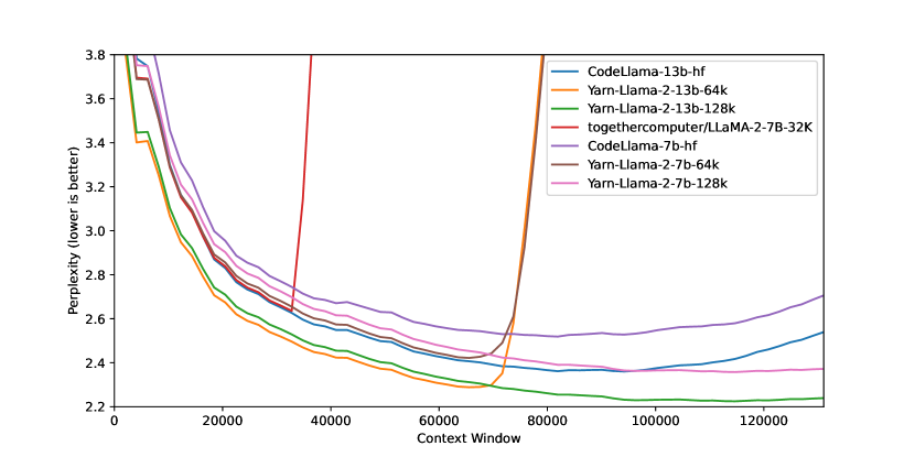
YaRN consistently outperforms both methods on long-context benchmarks (SCROLLS, LongBench) at the same scale, with less fine-tuning than linear interpolation.
Models Using YaRN
- Mistral 7B v0.2 (context extension from 8k to 32k)
- Qwen2 series (various context lengths)
- LLaMA-2 fine-tuned variants (community-produced 32k/64k/128k models)
YaRN is the standard method for context extension in the open-source community.
Comparison of Context Extension Methods
| Method | High-freq | Low-freq | Temperature | Fine-tune | Quality |
|---|---|---|---|---|---|
| Linear interp | Broken | Good | No | ~1000 steps | Moderate |
| NTK scaling | Good | Good | No | 0 | Good |
| NTK (dynamic) | Good | Good | No | 0 | Good |
| YaRN | Preserved | Good | Yes | ~400 | Best |
Summary
YaRN improves on earlier RoPE extension methods by:
- Treating different frequency bands differently (local, transitional, long-range)
- Correcting attention temperature to maintain focus at long context
- Requiring minimal fine-tuning (~400 steps)
It is the current community standard for extending the context of open-weight models, used in Mistral and many LLaMA derivatives.
References
- Peng, B., Quesnelle, J., Fan, H., & Shippole, E. (2023). YaRN: Efficient Context Window Extension of Large Language Models. ICLR 2024 (YaRN: combines NTK-Aware Scaling with attention temperature correction and frequency-interpolation to extend context with minimal fine-tuning).
- Su, J., Lu, Y., Pan, S., Murtadha, A., Wen, B., & Liu, Y. (2021). RoFormer: Enhanced Transformer with Rotary Position Embedding. arXiv 2021 (RoPE: the base positional encoding that YaRN extends for long-context models).
- Chen, S., Wong, S., Luo, L., & Tian, Y. (2023). Extending Context Window of Large Language Models via Positional Interpolation. arXiv 2023 (Position Interpolation: the predecessor approach that YaRN improves upon by addressing the frequency-dimension asymmetry).