
The Transformer Block: Putting It All Together
Published:
The Block is the Atom
The Transformer is not a complex monolith. It is a simple building block — the Transformer block — stacked repeatedly. GPT-2 small stacks 12. GPT-3 stacks 96. LLaMA 3 (70B) stacks 80. But each block is identical in structure.
Understand one block; understand any Transformer.
Data Flow: Token Embeddings
Before the first block, each input token is converted to a vector via an embedding lookup and summed with a positional encoding:
"The"  → embedding[The]  + pos_enc[0]  → x₀ ∈ ℝ^d_model
"cat"  → embedding[cat]  + pos_enc[1]  → x₁ ∈ ℝ^d_model
"sat"  → embedding[sat]  + pos_enc[2]  → x₂ ∈ ℝ^d_model
These vectors form a matrix X ∈ ℝ^{seq_len × d_model}. This matrix flows through the stack of blocks.
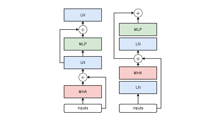
The Pre-LN Transformer Block (Modern Standard)
│ ├─── Identity copy ──────────────────────────────────────────── ⊕ ←──┐ │ │ └──→ LayerNorm → MultiHeadAttention ─────────────────────────────────────┘ ↓ x' (attended representation) │ ├─── Identity copy ──────────────────────────────────────────── ⊕ ←──┐ │ │ └──→ LayerNorm → FeedForward (MLP) ───────────────────────────────────┘ ↓ OUTPUT: x'' (shape: [seq_len, d_model])
In equations:
x'' = x' + FFN( LayerNorm(x') )
Two additions. Two layer norms. One attention operation. One FFN. That is the entire block.
Step-by-Step Walkthrough
Step 1: Layer Norm (before attention)
The input x is normalised across its feature dimension. Each token’s d_model-dimensional vector is scaled to zero mean and unit variance, then re-scaled by learned γ and β.
This stabilises the distribution entering attention, preventing runaway growth of attention logits.
Step 2: Multi-Head Attention
The normalised input is projected into Q, K, V for each head:
- Q, K used to compute attention weights (which tokens attend to which)
- V used to compute the attended output (what information is retrieved)
Heads run in parallel; their outputs are concatenated and projected back to d_model.
Output shape: [seq_len, d_model] — same as input.
Step 3: First Residual Addition
The attention output is added back to the original x (before normalisation). This is the residual connection:
x' = x + attention_output
The original signal is preserved. The attention result is a small correction to it.
Step 4: Layer Norm (before FFN)
The post-attention representation x’ is normalised again, feeding into the FFN with a well-conditioned distribution.
Step 5: Feed-Forward Network
The FFN processes each token position independently:
- Project up: d_model → 4 × d_model
- Nonlinearity: GELU or SwiGLU
- Project down: 4 × d_model → d_model
The FFN does not mix positions — it refines each token’s representation in place.
Step 6: Second Residual Addition
x'' = x' + ffn_output
The FFN’s contribution is added to x’. Again, the skip connection preserves the signal.
x’’ is the output of the block and becomes the input to the next block.
Shapes Throughout One Block
| Stage | Tensor shape |
|---|---|
| Input x | [L, d_model] |
| After LN (pre-attention) | [L, d_model] |
| Q, K per head | [L, d_k] each |
| V per head | [L, d_v] each |
| Attention output (per head) | [L, d_v] |
| After concat + project | [L, d_model] |
| After residual | [L, d_model] |
| After LN (pre-FFN) | [L, d_model] |
| After W₁ (FFN expand) | [L, 4·d_model] |
| After W₂ (FFN contract) | [L, d_model] |
| After residual (output) | [L, d_model] |
The shape is always [L, d_model] entering and leaving the block. Stacking blocks does not change the shape — only the content.
What Each Component Contributes
| Component | Role |
|---|---|
| Layer Norm | Stabilises distributions; enables deep stacking |
| Multi-Head Attention | Mixes information across positions |
| First Residual | Preserves input; enables gradient highway |
| Feed-Forward Network | Refines per-position; stores knowledge |
| Second Residual | Preserves input; enables gradient highway |
The Stack
A full Transformer is this block, repeated N times, followed by a final layer norm and an output head:
Token + Positional Embeddings
         ↓
   [Block 1]  ← LN → MHA → + → LN → FFN → +
         ↓
   [Block 2]
         ↓
      ...
         ↓
   [Block N]
         ↓
   Final LayerNorm
         ↓
   Output projection (lm_head): d_model → vocab_size
         ↓
   Logits → softmax → token probabilities
GPT-3 at 175B parameters is 96 of these blocks, each with d_model=12288, 96 attention heads, and d_ff=49152. The architecture is the same as described here. The only differences are scale and a few engineering choices (RoPE, SwiGLU, grouped-query attention in modern models).
Animated: Information Flow Through One Block
Why This Block Scales So Well
- The attention sub-layer mixes information globally across the sequence.
- The FFN sub-layer increases per-token expressivity without changing sequence length.
- Residuals let gradients bypass either sub-layer if needed.
- Layer norm keeps the statistics stable enough to stack dozens or hundreds of blocks.
That division of labor is why the same blueprint works from tiny classroom models to frontier LLMs.
Summary
The Transformer block is:
- LN + MHA + Residual — cross-position information gathering
- LN + FFN + Residual — per-position processing and knowledge retrieval
Everything else in a Transformer — BERT, GPT, T5, ViT, LLaMA — is a combination of how these blocks are arranged, what masking strategy is used, and what input/output heads are attached. The block itself is always the same.
References
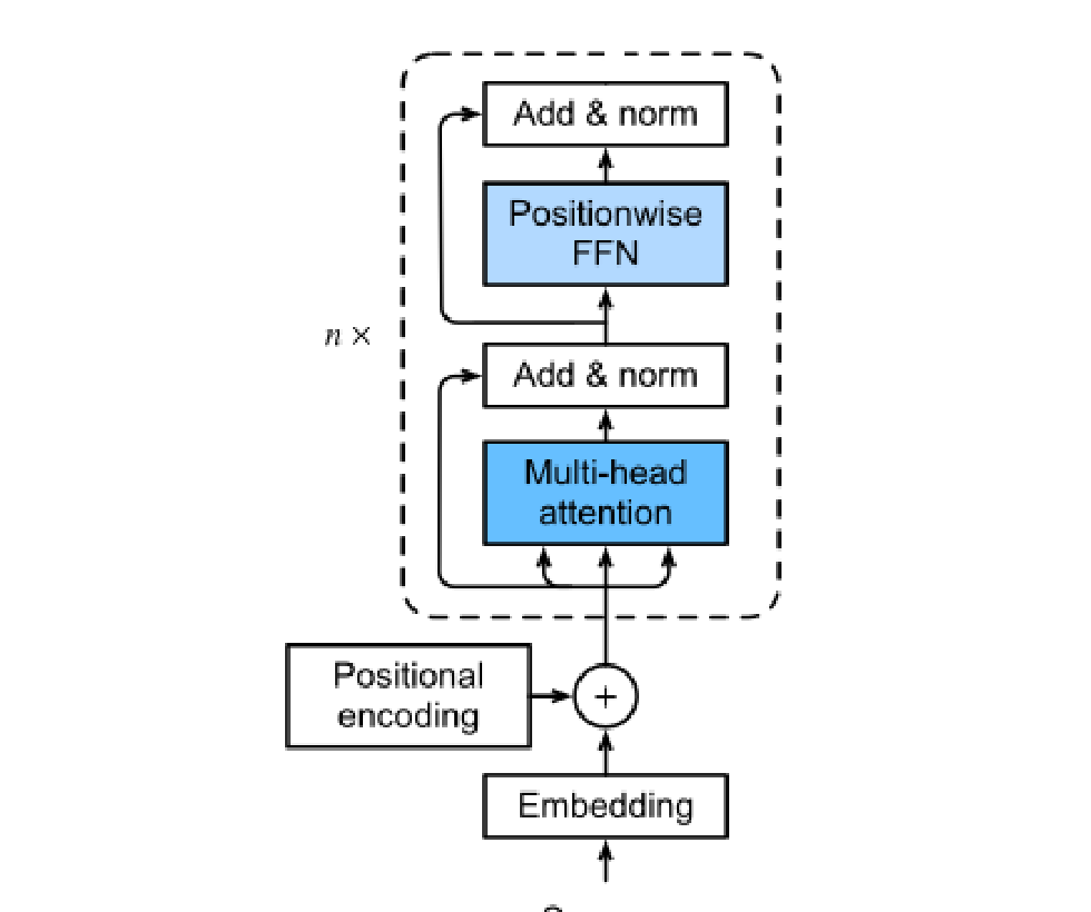
- Vaswani, A., Shazeer, N., Parmar, N., Uszkoreit, J., Jones, L., Gomez, A. N., Kaiser, Ł., & Polosukhin, I. (2017). Attention Is All You Need. NeurIPS 2017 (original Transformer block: MHA → Add&Norm → FFN → Add&Norm, stacked L times).
- Xiong, R., Yang, Y., He, D., Zheng, K., Zheng, S., Xing, C., Zhang, H., Lan, Y., Wang, L., & Liu, T.-Y. (2020). On Layer Normalization in the Transformer Architecture. ICML 2020 (Pre-LN block variant: LN before each sublayer instead of after — improves gradient flow and dominates modern LLM architectures).
- Geva, M., et al. (2021). Transformer Feed-Forward Layers Are Key-Value Memories.
- Touvron, H., Lavril, T., Izacard, G., Martinet, X., Lachaux, M.-A., Lacroix, T., Rozière, B., Goyal, N., Hambro, E., Azhar, F., Rodriguez, A., Joulin, A., Grave, E., & Lample, G. (2023). LLaMA: Open and Efficient Foundation Language Models. arXiv 2023 (LLaMA: uses Pre-LN block with RMSNorm, SwiGLU FFN, and RoPE — the dominant open-weight Transformer block design).
- [2] https://www.sscardapane.it/alice-book/