
Scaled Dot-Product Attention: Why the √d Matters
Published:
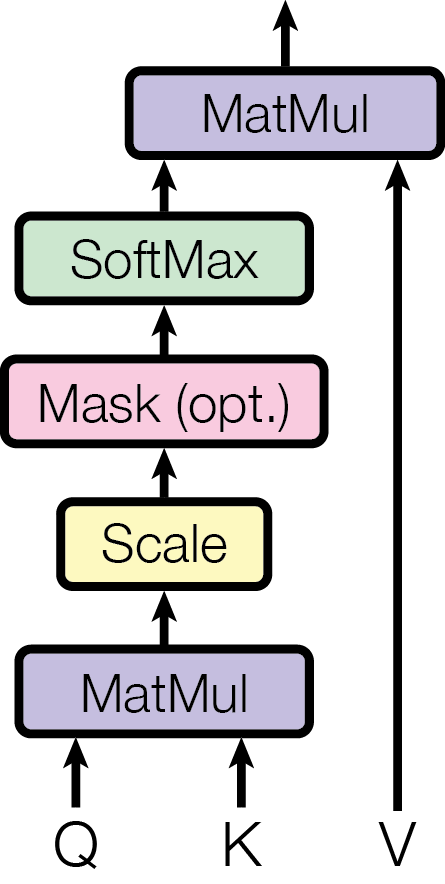
The Formula
Scaled dot-product attention is the engine inside every Transformer. Given queries Q, keys K, and values V:
The term \(d_k\) is the dimension of the key vectors. The division by \(\sqrt{d_k}\) is the “scaling” in the name. It looks minor. It is not.
Why Dot Products Grow in High Dimensions
Imagine two vectors \(q\) and \(k\), each of dimension \(d_k\), with components independently drawn from a standard normal distribution (mean 0, variance 1).
Their dot product \(q \cdot k = \sum_i q_i k_i\) has:
- Mean \(= 0\) (products of zero-mean variables)
- Variance \(= d_k\) (sum of \(d_k\) independent unit-variance terms)
So the standard deviation of the dot product grows as \(\sqrt{d_k}\).
When \(d_k = 64\) (a typical value), individual dot products have std \(\approx 8\). When \(d_k = 512\), std \(\approx 22\). As dimensions scale up, raw dot products naturally take on large absolute values.
What Happens to Softmax with Large Inputs
Softmax is defined as:
When inputs are large, say the vector \([35, 2, -10, 1]\), the exponential function amplifies differences exponentially. The largest value dominates completely. The output becomes something like \([\approx 1.0,\ \approx 0.0,\ \approx 0.0,\ \approx 0.0]\).
This is called softmax saturation. The “soft” maximum collapses into a hard argmax.
The Gradient Problem
Softmax saturation is catastrophic for learning because it causes gradient death. The gradient of softmax with respect to its input is:
When (\mathrm{softmax}(x_i) \approx 1), the factor ((1-\mathrm{softmax}(x_i))) is near zero. When (\mathrm{softmax}(x_i) \approx 0), the leading (\mathrm{softmax}(x_i)) term is near zero.
In both cases: no gradient flows. No learning happens. The attention weights are stuck.
The Fix: Divide by \(\sqrt{d_k}\)
Dividing each dot product by \(\sqrt{d_k}\) scales the variance back to 1:
Now the inputs to softmax live in a reasonable range regardless of \(d_k\). Softmax operates in its smooth, differentiable regime. Gradients flow. Learning works.
Why This Is So Easy to Miss
If you only read the attention formula once, the scaling term looks cosmetic. In reality it is a stability device: attention is not just about matching tokens, it is also about keeping those matches in a numerical regime where softmax can still learn.
Concrete Numerical Example
Suppose \(d_k = 64\) and two vectors \(q = k = [1/8, 1/8, \dots, 1/8]\) (all 64 entries equal 1/8).
Unscaled dot product:
q · k = 64 × (1/8 × 1/8) = 64 × 1/64 = 1.0
Now try \(q\) with entries drawn from \(N(0,1)\): typical magnitude \(\approx \sqrt{64} = 8\).
A score of 8 vs. −8 in a 4-token sequence:
softmax([8, -8, 2, -1]) ≈ [0.9997, 0.000, 0.003, 0.0001]
Nearly all weight on one token, a hard argmax. Gradient \(\approx 0\).
After scaling by \(\sqrt{64} = 8\):
softmax([1.0, -1.0, 0.25, -0.125]) ≈ [0.47, 0.06, 0.30, 0.17]
Smooth distribution. Gradient flows to all four tokens.
Visualising the Effect
| \(d_k\) | Raw std(\(q \cdot k\)) | Scaled std | Softmax regime |
|---|---|---|---|
| 4 | 2 | 1 | Smooth |
| 64 | 8 | 1 | Smooth |
| 512 | 22.6 | 1 | Smooth |
| 512 (unscaled) | 22.6 | 22.6 | Saturated |
Without scaling, increasing model width makes attention increasingly broken.
What About Other Scaling Choices?
Why \(\sqrt{d_k}\) specifically, and not \(d_k\) or some learned parameter?
- \(\div\, d_k\): over-shrinks; dot products become too small, softmax becomes too uniform (near-equal weights, no sharp attention)
- \(\div\, \sqrt{d_k}\): correct normalization that restores unit variance
- Learned scale: works in practice (some models do this), but adds parameters and can be poorly initialised
The \(\sqrt{d_k}\) formula hits the theoretical optimum for variance normalisation with minimal complexity.
Summary
| Without scaling | With scaling |
|---|---|
| Dot products grow as \(\sqrt{d_k}\) | Dot products stay \(\sim O(1)\) |
| Softmax saturates | Softmax is smooth |
| Gradients vanish | Gradients flow cleanly |
| Larger models train worse | Larger models train fine |
The \(\sqrt{d_k}\) is a single division that makes Transformers scalable. It is easy to overlook, but foundational to why the architecture works at all.
References
- Vaswani, A., Shazeer, N., Parmar, N., Uszkoreit, J., Jones, L., Gomez, A. N., Kaiser, Ł., & Polosukhin, I. (2017). Attention Is All You Need. NeurIPS 2017 (the original Transformer paper introducing scaled dot-product attention and multi-head attention).
- Bahdanau, D., Cho, K., & Bengio, Y. (2015). Neural Machine Translation by Jointly Learning to Align and Translate. ICLR 2015 (the additive attention mechanism that preceded scaled dot-product attention and motivated the QKV formulation).