
Residual Connections: Why Transformers Can Be Deep
Published:
Intuition First: The Highway Analogy
Picture a motorway with 96 exits in sequence. Without residual connections, information must travel through every exit in order — if one exit is blocked (saturated gradient), everything behind it grinds to a halt.
A residual connection adds a parallel express lane that bypasses each exit entirely. Traffic (gradients) can always reach the start of the motorway via the express lane, regardless of congestion at any individual exit.
The Problem with Deep Networks
Stacking many layers allows a model to learn increasingly abstract representations. But deep networks face a fundamental training problem: vanishing gradients.
During backpropagation, gradients are computed by repeated multiplication through the chain rule. In a network with L layers, the gradient of the loss with respect to early-layer weights involves multiplying L Jacobians together. If each Jacobian has singular values less than 1 (common for standard activations), the gradient shrinks exponentially. Early layers learn almost nothing.
This is why naive deep networks (without tricks) perform worse than shallower ones — a counter-intuitive result that motivated residual connections.
The Residual Fix
Introduced by He et al. (2015) for CNNs (ResNet), residual connections add the input directly to the output of each sub-layer:
Where x is the input, f(x) is whatever the sub-layer computes (attention, FFN, etc.), and y is the output.
This changes what the sub-layer must learn. Instead of learning a full transformation from x to the desired output, it only needs to learn the residual — the difference between x and the desired output. If no change is needed, f(x) = 0 works perfectly (identity function).
Why Gradients Flow Better
In a standard deep network, the gradient of the loss L with respect to an early activation x_l is:
This is a product of L Jacobians — exponentially small or large.
With residual connections, y_l = x_l + f(x_l), so:
The gradient always includes the 1 term — a direct, unattenuated path from output to input. Even if ∂f/∂x_l ≈ 0 (a saturated or poorly-conditioned sub-layer), the gradient still flows back as 1.
Summing over all paths: gradients reach early layers directly via the skip connections. Deep networks become trainable.
Residuals as Incremental Refinements
The residual formulation y = x + f(x) has another interpretation: each layer proposes a small correction to the current representation.
If f is initialised near zero (which happens naturally with small random weights), then at the start of training y ≈ x. The network begins as a near-identity function — a useful initialisation since the untrained network does not corrupt the signal.
As training progresses, each layer learns to add increasingly meaningful corrections. This is why Transformers initialise stably even at 96 layers — no single layer needs to do anything dramatic from the start.
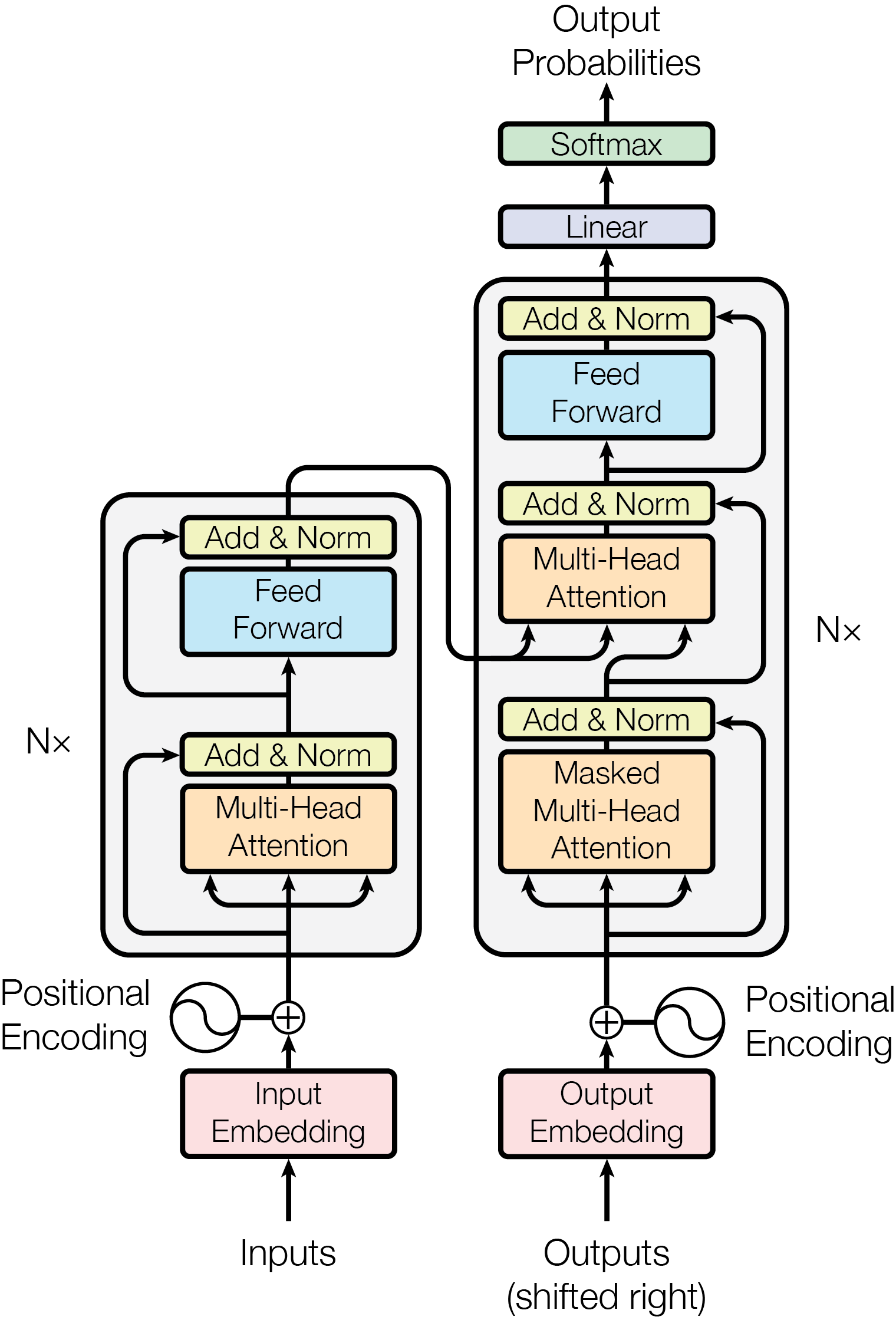
In Transformers: Two Residuals per Block
Each Transformer block contains two sub-layers (attention and FFN), each with its own residual connection:
┌─────────────────────────────────────────────┐
│  x ──────────────────────────────────────+  │
│  │                                       │  │
│  └→ LayerNorm → MultiHeadAttention ─────┘  │
│                                             │
│  x' ─────────────────────────────────────+ │
│  │                                       │ │
│  └→ LayerNorm → FeedForward ────────────┘ │
└─────────────────────────────────────────────┘
GPT-3’s 96 layers means 192 residual additions. At every single one, there is a direct gradient highway from the loss all the way back to the input.
The Residual Stream View
A useful mental model: think of the Transformer as a residual stream — a single high-dimensional vector that persists across all layers. Each attention head and FFN block reads from this stream and writes back to it via residual addition.
This view, popularised by mechanistic interpretability research (Elhage et al., 2021), makes it clear that:
- Information is preserved across layers (it stays in the stream)
- Each layer adds information rather than replacing it
- Individual layers can be interpreted as reading/writing to a shared memory
Concrete Example: Gradient Flow with and Without Residuals
Consider a toy 3-layer network, each layer applying a transformation with Jacobian magnitude 0.5:
Without residuals:
Gradient reaching layer 1 = 1 × 0.5 × 0.5 × 0.5 = 0.125
After 10 layers: 1 × 0.5^10 ≈ 0.001 — essentially vanished.
With residuals (each Jacobian is now 1 + 0.5 = 1.5 at best, but more importantly the identity term always contributes 1):
Even if ∂f/∂x ≈ 0 at every layer, gradient at layer 1 = 1.0 (via the skip path).
In practice the Jacobian is (1 + small correction), so even 96 layers multiply out to a value near 1 rather than near zero.
This is the key: the “1” in (1 + ∂f/∂x) acts as a floor that prevents gradient collapse.
What Happens Without Residuals?
Ablation studies confirm: removing residual connections from deep Transformers causes:
- Training instability (loss spikes, divergence)
- Significantly worse final performance
- Requirement for much more careful learning rate tuning
Adding them back is cheap — it is a single addition with no parameters — but the effect is profound.
Summary
| Without residuals | With residuals |
|---|---|
| Gradients vanish in early layers | Gradients flow via identity skip |
| Layers learn full transformations | Layers learn small refinements |
| Deep networks hard to train | Deep networks train stably |
| Initialisation is fragile | Initialisation is near-identity |
| Performance degrades with depth | Performance improves with depth |
Residual connections are the single most important structural element that allows Transformers to scale to hundreds of layers. They cost almost nothing (one addition) but change everything.
References
- He, K., Zhang, X., Ren, S., & Sun, J. (2016). Deep Residual Learning for Image Recognition. CVPR 2016 (ResNets: introduced residual skip connections to train very deep networks; adopted directly into Transformers by Vaswani et al.).
- Vaswani, A., Shazeer, N., Parmar, N., Uszkoreit, J., Jones, L., Gomez, A. N., Kaiser, Ł., & Polosukhin, I. (2017). Attention Is All You Need. NeurIPS 2017 (Transformer: uses Add & Norm (residual + layer norm) after both attention and FFN sublayers in each block).
- Veit, A., Wilber, M., & Belongie, S. (2016). Residual Networks Behave Like Ensembles of Relatively Shallow Networks. NeurIPS 2016 (shows residual networks create exponentially many paths of varying length, explaining their robustness to layer removal).