
Layer Normalization in Transformers
Published:
Intuition First: What Does “Normalise” Actually Do?
Imagine you are a neuron receiving thousands of inputs from the previous layer. If those inputs have wildly different scales — some near 0, some near 1000 — your weights need to be tiny for large inputs and large for small inputs simultaneously. That is a frustrating optimisation landscape.
Normalisation is simply: “before passing information to the next layer, rescale it so every token’s feature vector looks roughly the same.” You lose no information (learned γ and β can undo the normalisation) but you gain a predictable, well-conditioned signal at every layer.
Why Normalisation at All?
Deep networks suffer from internal covariate shift: as weights update during training, the distribution of activations at each layer changes unpredictably. Later layers must constantly adapt to a moving target.
Normalisation layers stabilise these distributions. For Transformers, layer normalisation is the standard solution.
Layer Norm vs Batch Norm
Batch Normalisation normalises across the batch dimension: for each feature, compute mean and variance across all examples in the batch.
- Problematic for variable-length sequences (different batch elements have different lengths)
- Requires large batch sizes to estimate statistics reliably
- Behaviour differs between training and inference (running mean/var at test time)
Layer Normalisation normalises across the feature dimension: for each token, compute mean and variance across all d_model features.
- Independent of batch size and sequence length
- Identical behaviour at training and inference time
- Natural fit for sequence models
The Layer Norm Formula
Given a token representation x ∈ ℝ^d:
LayerNorm(x) = γ · (x − μ) / √(σ² + ε) + β
- μ, σ² are computed per-token (across features)
- γ (scale) and β (shift) are learned parameters, initialised to 1 and 0 respectively
- ε (typically 1e-5) prevents division by zero
After normalisation, the output has approximately zero mean and unit variance. γ and β then allow the network to re-scale and re-shift to whatever distribution is optimal — without collapsing the normalisation.
Worked Example: LayerNorm on a 4-Dimensional Token
Suppose a token’s representation is x = [2, 4, −2, 0] (d = 4, simplified).
Step 1 — Compute mean:
μ = (2 + 4 + (−2) + 0) / 4 = 1.0
Step 2 — Compute variance:
σ² = [(2−1)² + (4−1)² + (−2−1)² + (0−1)²] / 4
= [1 + 9 + 9 + 1] / 4 = 5.0
Step 3 — Normalise:
x̂ = (x − μ) / √(σ² + ε) ≈ [1/√5, 3/√5, −3/√5, −1/√5] ≈ [0.45, 1.34, −1.34, −0.45]
Step 4 — Apply γ and β (assume γ = [1,1,1,1], β = [0,0,0,0] at initialisation):
Output = γ · x̂ + β = [0.45, 1.34, −1.34, −0.45]
After training, γ and β may have become [2, 1, 1, 0.5] and [0.1, −0.2, 0.1, 0] — allowing the network to recover any useful scale it needs while keeping the normalisation benefit.
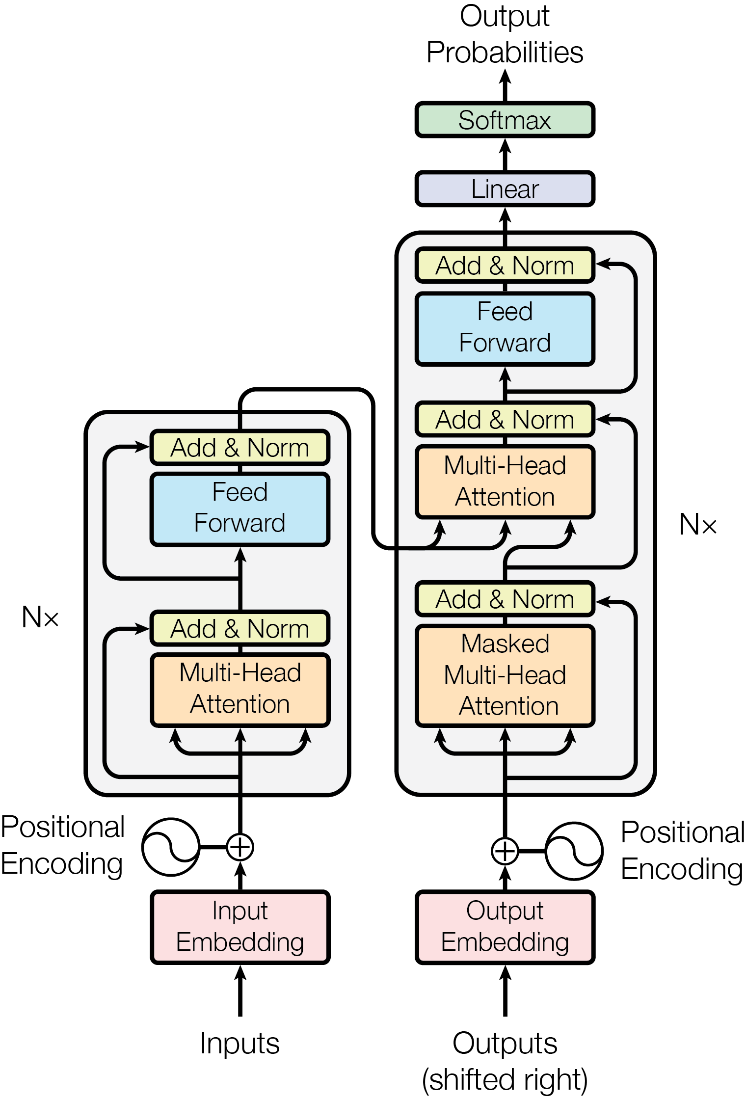
Post-LN: The Original Placement
The 2017 Transformer paper placed layer norm after the residual addition:
In full notation for one sub-layer:
y = LayerNorm(x + Sublayer(x))
This is called Post-LN (normalisation after the residual). It was the standard until roughly 2019.
Problem: In Post-LN, gradients must flow through the LayerNorm on the path back through the residual stream. At initialisation, this can produce very large or unstable gradients in early layers of deep networks. Post-LN models require careful learning rate warmup and are sensitive to hyperparameters.
Pre-LN: The Modern Standard
Pre-LN places layer norm before each sub-layer, inside the residual branch:
In full notation:
y = x + Sublayer(LayerNorm(x))
The residual path remains a clean identity: y = x + f(x). Gradients can bypass the sub-layer entirely by flowing through the residual skip connection. This dramatically stabilises training.
RMSNorm: A Simpler Variant
Many recent models (LLaMA, Mistral, Gemma) use RMSNorm instead of full layer norm:
RMSNorm removes the mean-centering step (no μ subtraction). This is:
- Faster: ~15-20% less computation
- Equally effective empirically
- Motivated by the observation that re-centring contributes little to training stability
The scale γ is still learned; the shift β is dropped.
Where LayerNorm Appears in a Transformer Block
In a Pre-LN Transformer, each block looks like:
x → LN → MultiHeadAttention → + x → LN → FFN → + x
          ↑___________________↑       ↑__________↑
               residual                 residual
There are two layer norms per block: one before attention, one before the FFN. For a 96-layer model (GPT-3 scale), that is 192 LayerNorm operations per forward pass.
Comparison
| Property | Post-LN | Pre-LN | RMSNorm |
|---|---|---|---|
| Gradient flow | Through LN | Via identity skip | Via identity skip |
| Training stability | Lower | Higher | Higher |
| Warmup required | Usually yes | Often no | Often no |
| Used by | BERT, original T5 | GPT-2/3, LLaMA | LLaMA 2/3, Mistral |
| Mean-centering | Yes | Yes | No |
| Compute | Standard | Standard | ~15% faster |
Summary
Layer norm is not cosmetic. It controls how information flows and how gradients propagate through the network. The choice between Pre-LN and Post-LN explains many practical differences between model families — and Pre-LN’s superior stability is why it dominates modern large language model training.
References
- Ba, J. L., Kiros, J. R., & Hinton, G. E. (2016). Layer Normalization. arXiv 2016 (LayerNorm: normalises across the feature dimension rather than the batch dimension, enabling stable training of sequence models).
- Xiong, R., Yang, Y., He, D., Zheng, K., Zheng, S., Xing, C., Zhang, H., Lan, Y., Wang, L., & Liu, T.-Y. (2020). On Layer Normalization in the Transformer Architecture. ICML 2020 (Pre-LN vs Post-LN: theoretical and empirical comparison showing Pre-LN (before attention) improves gradient flow and training stability).
- Zhang, B., & Sennrich, R. (2019). Root Mean Square Layer Normalization. NeurIPS 2019 (RMSNorm: removes the mean-centering step from LayerNorm — used in LLaMA, Mistral, and most modern open-weight LLMs).