
Message Passing on Simplicial Complexes
Published:
The distinction a graph cannot make
Draw three vertices and join them into a cycle. Now ask: is that a loop, or is it a filled patch of surface with a loop for a border?
A graph has no way to answer. A graph is a set of vertices and a set of pairs; there is no third slot in which to record that the interior has been filled in. Every graph neural network you can write, no matter how deep, receives exactly the same input in both cases, and so must produce the same output. This is not an expressivity failure of any particular architecture. The information was never in the data structure.
A simplicial complex has that third slot, and a fourth, and so on. The point of this post is the mechanism: how message passing generalises once the domain contains cells of every dimension, and what specifically it buys you. The short answer is that a single notion of “neighbour” splits into four, and the interesting one, upper adjacency, is precisely the one that notices the filling.
The domain
An abstract simplicial complex \(K\) on a vertex set \(V\) is a collection of non-empty finite subsets of \(V\) that is closed under taking subsets: if \(\sigma \in K\) and \(\emptyset \neq \tau \subseteq \sigma\), then \(\tau \in K\). An element \(\sigma \in K\) with \(\lvert \sigma \rvert = p+1\) is a \(p\)-simplex, or a \(p\)-cell. So vertices are \(0\)-cells, edges are \(1\)-cells, triangles are \(2\)-cells, tetrahedra are \(3\)-cells.
The closure condition is the whole content. It says a triangle cannot be present unless all three of its edges are, and none of its edges unless all of its vertices are. A complex is a graph plus permission to declare some of its cliques filled.
We write \(\tau \prec \sigma\) when \(\tau \subset \sigma\) and \(\dim \tau = \dim \sigma - 1\): \(\tau\) is a face of \(\sigma\), and \(\sigma\) a coface of \(\tau\). A \(p\)-cell has exactly \(p+1\) faces; it may have any number of cofaces, including none.
The learning setup differs from the graph case in one respect that drives everything else. Features do not live only on vertices. Every cell carries one:
with the dimension of the feature space allowed to depend on \(p\), since edge features and triangle features need not mean the same thing. A layer maps the whole collection \(\{h_\sigma\}_{\sigma \in K}\) to a new one.
A complex small enough to enumerate
Here is the example the rest of the post runs on. Take four vertices and this complex:
writing \(12\) for \(\{1,2\}\) and so on. Ten cells in total: four vertices, five edges, one triangle. Check the closure condition on the only \(2\)-cell: the faces of \(123\) are \(12\), \(13\), \(23\), all present.
The underlying graph contains two triangular cycles, \(1\!-\!2\!-\!3\) and \(2\!-\!3\!-\!4\). Only the first is filled. As a graph the two are indistinguishable by any local rule; as a complex they are different, and the difference is a single element of \(K_2\). Everything below is a way of making a network feel that difference.
Why four neighbourhoods
Fix a \(p\)-cell \(\sigma\). There are four natural ways for another cell to be near it, and they are genuinely different relations, not one relation described four times.
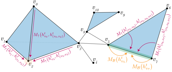
Boundary. \(\mathcal{B}(\sigma) = \{ \tau \in K : \tau \prec \sigma \}\), the \((p-1)\)-faces of \(\sigma\). This looks down a dimension. For \(\sigma = 123\) the boundary is \(\{12, 13, 23\}\); a triangle hears from its own edges.
Coboundary. \(\mathcal{C}(\sigma) = \{ \delta \in K : \sigma \prec \delta \}\), the \((p+1)\)-cells having \(\sigma\) as a face. This looks up. For \(\sigma = 12\) the coboundary is \(\{123\}\); the edge hears from the triangle it helps bound. For \(\sigma = 24\) the coboundary is empty.
Lower adjacency. \(\mathcal{N}_{\downarrow}(\sigma) = \{ \tau \in K : \dim \tau = p,\ \tau \neq \sigma,\ \exists\, \rho \text{ with } \rho \prec \sigma \text{ and } \rho \prec \tau \}\). Two \(p\)-cells are lower-adjacent when they share a face. Two edges are lower-adjacent when they share a vertex.
Upper adjacency. \(\mathcal{N}_{\uparrow}(\sigma) = \{ \tau \in K : \dim \tau = p,\ \tau \neq \sigma,\ \exists\, \delta \in K \text{ with } \sigma \prec \delta \text{ and } \tau \prec \delta \}\). Two \(p\)-cells are upper-adjacent when they are both faces of one common \((p+1)\)-cell. Two edges are upper-adjacent when some filled triangle contains both.
Why not merge them? Because a message from a face and a message from a coface are messages from different kinds of object, arriving from different directions in the dimension hierarchy, and they should be allowed different weights. Merging them would be like a graph network that adds incoming and outgoing messages on a directed graph and forgets which was which. More sharply: the four relations are not redundant. The examples below show two cells with identical lower adjacency and different upper adjacency, and that difference is exactly the topological content.
Worked out on \(K\)
Take the edge \(\sigma = 12\):
- \(\mathcal{B}(12) = \{1, 2\}\), its two endpoints.
- \(\mathcal{C}(12) = \{123\}\), one triangle.
- \(\mathcal{N}_{\downarrow}(12) = \{13, 23, 24\}\), \(13\) shares vertex \(1\); \(23\) and \(24\) share vertex \(2\). Note \(34\) is absent: it shares no endpoint with \(12\).
- \(\mathcal{N}_{\uparrow}(12) = \{13, 23\}\), the other two faces of \(123\).
Now take the edge \(\sigma = 24\):
- \(\mathcal{B}(24) = \{2, 4\}\).
- \(\mathcal{C}(24) = \emptyset\), no triangle of \(K\) contains it.
- \(\mathcal{N}_{\downarrow}(24) = \{12, 23, 34\}\), \(12\) and \(23\) share vertex \(2\); \(34\) shares vertex \(4\).
- \(\mathcal{N}_{\uparrow}(24) = \emptyset\).
Both edges have exactly three lower neighbours. One has two upper neighbours, the other none. That is the asymmetry. Compare the pair \((12, 13)\) with the pair \((24, 34)\): in each case two edges meeting at a vertex, in each case part of a triangular cycle in the graph. The first pair is upper-adjacent, the second is not, because \(123 \in K\) and \(234 \notin K\). A graph neural network sees the two pairs as locally identical configurations. Upper adjacency is the channel through which the fill becomes visible.
Two more, for the boundary rows of the scheme. For the vertex \(\sigma = 1\): \(\mathcal{B}(1) = \emptyset\) (a \(0\)-cell has no faces), \(\mathcal{C}(1) = \{12, 13\}\), \(\mathcal{N}_{\downarrow}(1) = \emptyset\) (vertices share no faces), and \(\mathcal{N}_{\uparrow}(1) = \{2, 3\}\), which is exactly the graph neighbourhood of vertex \(1\). Hold on to that. For the triangle \(\sigma = 123\): \(\mathcal{B} = \{12, 13, 23\}\), and \(\mathcal{C}\), \(\mathcal{N}_{\downarrow}\), \(\mathcal{N}_{\uparrow}\) are all empty, since \(K\) has no \(3\)-cells and no other \(2\)-cells.
The update rule
Each neighbourhood produces one message, aggregated over that neighbourhood with a permutation-invariant operator (sum, mean, max), and the four are combined with the cell’s own feature. Writing \(M\) for learned message functions, \(\bigoplus\) for the aggregator and \(U\) for the update:
Three details are worth pausing on.
The message functions carry a subscript. \(M_{\mathcal{B}} \neq M_{\uparrow}\): separate parameters per relation, which is the entire reason for distinguishing the relations in the first place. In practice one also uses separate parameters per dimension \(p\), since the four functions acting on edges have a different job from the four acting on triangles.
The adjacency messages take a third argument. When \(\tau\) and \(\sigma\) are lower-adjacent, \(\sigma \cap \tau\) is the shared face, and it is a cell of \(K\) with a feature of its own; when they are upper-adjacent, \(\sigma \cup \tau\) is the shared coface. Passing that feature in lets the network condition on what the two cells share, not merely that they share something. For \(p = 1\), the lower message from \(12\) to \(13\) is conditioned on the feature of vertex \(1\), and the upper message on the feature of triangle \(123\).
Some of the four are structurally empty for cells at the extremes. Vertices have no boundary and no lower adjacency; top-dimensional cells have no coboundary and no upper adjacency. Implementations pass a zero vector or a learned null embedding.
The graph case is the bottom row
Restrict to \(p = 0\) and keep only the upper message. As computed above, \(\mathcal{N}_{\uparrow}(v)\) is the set of graph neighbours of \(v\), and for \(u \in \mathcal{N}_{\uparrow}(v)\) the shared coface \(v \cup u\) is the edge \(uv\). The rule collapses to
which is message passing with edge features, unchanged. So this is not a different paradigm bolted on beside graph neural networks. It is the same recursion with the dimension index freed, and the familiar case sitting on the bottom row. Everything above \(p=0\) is new capacity; nothing below it is lost.
Boundary maps, and the two Laplacians hiding in the scheme
The lower/upper split is not an ad-hoc modelling choice. It is the algebraic structure of the complex, and the connection is worth making precise because it tells you the two channels are measuring genuinely different things.
Orient each simplex by fixing an ordering of its vertices, here, increasing index. The boundary operator \(\partial_p\) maps oriented \(p\)-chains to \((p-1)\)-chains by the alternating sum
with \(\widehat{v_i}\) meaning that vertex is deleted. As a matrix, \(\partial_p\) has one row per \((p-1)\)-cell and one column per \(p\)-cell.
Verifying \(\partial_1 \partial_2 = 0\) on \(K\)
Order the edges \(12, 13, 23, 24, 34\) and the vertices \(1, 2, 3, 4\). The only \(2\)-cell gives
and \(\partial_1 [u,v] = [v] - [u]\) gives
Multiplying is one linear combination of columns, column \(12\) minus column \(13\) plus column \(23\):
Zero, as required. The identity \(\partial_p \partial_{p+1} = 0\) is what makes the sequence of chain groups a chain complex, and it holds for the reason visible here: every \((p-1)\)-face of a \(p{+}1\)-cell is reached along exactly two paths, with opposite signs.
The Hodge Laplacian splits the same way
The \(p\)-th Hodge Laplacian is
The naming is not a coincidence. Off the diagonal, \(L_p^{\uparrow}\) is supported exactly on upper-adjacent pairs and \(L_p^{\downarrow}\) exactly on lower-adjacent pairs, the two sparsity patterns are the two adjacency relations, up to sign. At \(p = 0\), where \(\partial_0 = 0\), we get \(L_0 = \partial_1 \partial_1^{\top}\), the ordinary graph Laplacian, consistent with the bottom row again.
On \(K\), the upper part is the outer product of \(\partial_2\) with itself:
The rows for \(24\) and \(34\) vanish. The empty triangle \(2\!-\!3\!-\!4\) contributes nothing to the upper Laplacian, while the filled triangle \(123\) couples its three edges. Same picture as the neighbourhood enumeration, now as a matrix.
There is a lesson in the sum, too. Take the pair \((12, 13)\). Its upper entry is \((+1)(-1) = -1\). Its lower entry is the inner product of the two columns of \(\partial_1\), namely \((-1,1,0,0) \cdot (-1,0,1,0) = 1\). They cancel: \((L_1)_{12,13} = 0\). The same happens for the other two pairs of edges in the filled triangle, and indeed \(L_1\) restricted to those three edges is \(3I\), no off-diagonal coupling at all, and no kernel, matching the fact that a filled triangle has no one-dimensional hole. Delete the \(2\)-cell and \(L_1\) on those edges becomes \(\partial_1^\top \partial_1\) alone, which annihilates the cycle \([1,2] - [1,3] + [2,3]\) and so has a one-dimensional kernel: the loop is back.
A note on orientation. The boundary maps and the Hodge Laplacian require a choice of orientation, and a different choice conjugates them by a diagonal sign matrix. The message-passing rule above uses no orientation at all, it works with unordered cells and their features. The two views are compatible: orientation is bookkeeping needed to write the operators, and the relations \(\mathcal{B}, \mathcal{C}, \mathcal{N}_{\downarrow}, \mathcal{N}_{\uparrow}\) that message passing consumes are orientation-free.
Expressivity, stated carefully
Graph neural networks that pass messages along edges are bounded above by the 1-dimensional Weisfeiler–Leman test: if 1-WL assigns two graphs the same colour histogram, no such network can separate them. This is a real ceiling and there are small graphs that sit on it.
The standard example: let \(G_1\) be the \(6\)-cycle and \(G_2\) the disjoint union of two triangles. Both have six vertices, six edges, and every vertex of degree \(2\). 1-WL starts with all vertices the same colour and refines by the multiset of neighbour colours, which is the same multiset, at every round, for every vertex of both graphs. The colourings never separate, and no amount of depth or width helps.
Now lift each graph to its clique complex: fill in every clique. In \(G_1\), the neighbours of any vertex are non-adjacent, so there are no \(3\)-cliques and the lift adds nothing, \(6\) vertices, \(6\) edges, \(0\) triangles, \(12\) cells. In \(G_2\), each triangle is a \(3\)-clique, so both get filled, \(6\) vertices, \(6\) edges, \(2\) triangles, \(14\) cells. After a single round of message passing, every edge of \(G_2\) has two upper neighbours and a non-empty coboundary; every edge of \(G_1\) has neither. The features diverge immediately, and any readout over cells separates the two.
It is worth being precise about what this shows and what it does not.
Two consequences follow. First, the lift decides what you can see. A clique complex makes cliques visible; it will not help with structure that is not clique-shaped, and other lifts, from rings in a molecule, say, or from a cover, expose other things. Second, the choice is a modelling assumption with the same status as choosing an architecture, and it can be wrong for the task: filling in every clique of a social graph asserts that dense groups are solid objects, which may be exactly backwards if the interesting signal is which groups are not closed.
The figure above draws only two of the four messages, upper and boundary. It is a reasonable guess from the figure that those two carry the expressive content and the other two are, at least for some purposes, redundant given them, but I have not verified the precise statement, so I am not claiming it.
What it costs
Plainly: the number of cells can explode, and the explosion is the point of failure.
The clique complex of the complete graph \(K_n\) contains every non-empty subset of the \(n\) vertices, so it has
cells. At \(n = 20\) that is \(1{,}048{,}575\) cells for a graph with \(20\) vertices and \(190\) edges. This is not a pathological input; it is a single dense community.
The usual mitigation is to truncate at dimension \(2\), keeping only vertices, edges and triangles, which caps the count at \(n + \binom{n}{2} + \binom{n}{3}\), cubic rather than exponential, but still cubic. And cell count is not the whole cost, since message passing runs over pairs: the lower-adjacency message for edges runs over pairs of edges sharing a vertex, of which a vertex of degree \(d\) contributes \(\binom{d}{2}\). High-degree hubs are expensive in a way they are not for a graph network, where a hub costs \(d\) and not \(d^2\).
Three further costs, none of them hidden:
- Memory scales with cells, not vertices. A \(d\)-dimensional feature on every triangle can dominate the vertex features outright.
- Preprocessing is real work. Enumerating cliques is not free, and it must be done before training, per graph.
- More parameters per layer. Four message functions per dimension, times the dimensions kept. On small datasets that is a variance problem, not a capacity win.
✅ Key Takeaways
- A simplicial complex stores cells of every dimension and features live on all of them, so a layer maps \(\{h_\sigma\}\) over the whole complex, not just over vertices.
- A \(p\)-cell has four neighbourhoods, boundary, coboundary, lower adjacency, upper adjacency, and they are separate relations with separate learned message functions.
- On the worked complex, edges \(12\) and \(24\) both have three lower neighbours, but \(12\) has two upper neighbours and \(24\) has none: the filled triangle \(123\) is in \(K\), the cycle \(2\!-\!3\!-\!4\) is not filled. That gap is the information a graph cannot represent.
- Setting \(p = 0\) and keeping only the upper message recovers graph message passing with edge features exactly.
- \(\partial_1 \partial_2 = 0\) was verified directly on the example, and the up/down split of \(L_p = \partial_{p+1}\partial_{p+1}^\top + \partial_p^\top \partial_p\) has the same sparsity patterns as upper/lower adjacency. The two parts can cancel, for the filled triangle they cancel to \(3I\), which is a reason to keep the message channels separate rather than working with \(L_p\) alone.
- The \(6\)-cycle and two disjoint triangles are 1-WL equivalent, but their clique complexes have \(0\) and \(2\) triangles respectively and separate after one round. The gain comes from the lift changing the input, not from a stronger refinement of the same input.
- The clique complex of \(K_n\) has \(2^n - 1\) cells. Truncating at dimension \(2\) makes it cubic; lower-adjacency messages still cost \(\binom{d}{2}\) at a degree-\(d\) vertex.
References
- Bodnar, C., Frasca, F., Wang, Y. G., Otter, N., Montúfar, G., Liò, P., & Bronstein, M. (2021). Weisfeiler and Lehman Go Topological: Message Passing Simplicial Networks. ICML 2021.
- Bodnar, C., Frasca, F., Otter, N., Wang, Y. G., Liò, P., Montúfar, G., & Bronstein, M. (2021). Weisfeiler and Lehman Go Cellular: CW Networks. NeurIPS 2021.
- Xu, K., Hu, W., Leskovec, J., & Jegelka, S. (2019). How Powerful are Graph Neural Networks? ICLR 2019.
- Lim, L.-H. Hodge Laplacians on Graphs. SIAM Review (arXiv:1507.05379).
- Barbarossa, S., & Sardellitti, S. (2020). Topological Signal Processing over Simplicial Complexes. IEEE Transactions on Signal Processing.
- Papillon, M., Sanborn, S., Hajij, M., & Miolane, N. (2023). Architectures of Topological Deep Learning: A Survey of Message-Passing Topological Neural Networks. arXiv:2304.10031.