The Weisfeiler-Lehman Test: How Powerful Are GNNs?

Intuition First: Why Can GNNs Fail to Tell Graphs Apart?

Imagine two cities with different road layouts but where every intersection has exactly the same number of roads connecting to it (i.e., regular graphs). If you stand at any intersection and look only at the local road count, every intersection looks identical — you cannot tell the cities apart without a map. A GNN operating by local neighbourhood aggregation faces the same problem: if two graphs have identical local multiset statistics at every scale, the GNN sees the same numbers everywhere and produces identical outputs.

The WL test formalises exactly which graph pairs fall into this trap.

What Is Graph Isomorphism?

Two graphs \(G\) and \(G'\) are isomorphic (\(G \cong G'\)) if there exists a bijection \(\sigma : V(G) \to V(G')\) such that \((u,v) \in E(G) \iff (\sigma(u), \sigma(v)) \in E(G')\). Informally: they are the same graph up to node relabelling.

Graph isomorphism testing is a fundamental problem. It is in NP, but is not known to be either in P or NP-complete — it sits in the small class of problems suspected to be of intermediate difficulty. For practical purposes, the 1-WL algorithm provides a fast, powerful, but incomplete test.

The 1-WL Algorithm (Colour Refinement)

Initialisation: assign every node the same colour \(c_v^{(0)}\), or a colour derived from its initial feature. (If all nodes start identical, the first iteration effectively colours by degree.)

Iteration: at step \(k\), each node \(v\) updates its colour by hashing its own previous colour together with the multiset of its neighbours’ previous colours:

where \(\mathcal{N}(v)\) is the neighbourhood of \(v\) and \(\{\!\{\cdot\}\!\}\) denotes a multiset — counts matter, order does not — and \(\mathrm{HASH}\) is injective, so two nodes receive the same new colour exactly when their (own colour, neighbour multiset) pairs agree.

Termination: stop when the partition of nodes into colour classes stops changing. This happens after at most \(N-1\) iterations, since the partition refines strictly at each step until it stabilises.

Test: compare the histograms of final colours of \(G\) and \(G'\).

• Histograms differ \(\Rightarrow\) \(G \not\cong G'\). This direction is sound: the test never reports a false negative for isomorphism.
• Histograms match \(\Rightarrow\) inconclusive. The graphs may or may not be isomorphic. It is common but sloppy to say 1-WL “declares them isomorphic”; all it can honestly report is that it failed to separate them.

Concrete Worked Example: Running 1-WL

Consider two graphs:

• \(G_1\): a triangle (3-cycle) A–B–C–A, all nodes of degree 2
• \(G_2\): three disjoint edges A–B, C–D, E–F (6 nodes, all of degree 1)

Iteration 1: starting from a uniform colouring, the first refinement separates nodes by degree.

• \(G_1\): every node gets the colour “deg 2” → histogram \(\{\!\{\text{deg2}: 3\}\!\}\)
• \(G_2\): every node gets the colour “deg 1” → histogram \(\{\!\{\text{deg1}: 6\}\!\}\)

The histograms differ, so 1-WL correctly certifies \(G_1 \not\cong G_2\). ✓ (Node counts alone would have settled this one.)

Now consider a genuinely hard pair, both on 6 nodes and 6 edges:

• \(G_3\): two disjoint triangles (all degree 2)
• \(G_4\): a 6-cycle A–B–C–D–E–F–A (all degree 2)

Iteration 1: both have histogram \(\{\!\{\text{deg2}: 6\}\!\}\). Same.

Iteration 2: each node hashes its colour with its neighbours’ colour multiset. In \(G_3\) every node has exactly two neighbours, both coloured “deg2”; in \(G_4\) the same. Every node’s input to \(\mathrm{HASH}\) is identical in both graphs, so the colouring is already stable and no further iteration changes anything.

1-WL therefore cannot distinguish \(G_3\) from \(G_4\) — and by the theorem below, neither can any MPNN, even though the graphs are plainly non-isomorphic (\(G_3\) is disconnected and full of triangles; \(G_4\) is connected and triangle-free).

This is the general phenomenon behind regular graphs: on any \(k\)-regular graph with uniform initial features, all nodes are permanently the same colour, so the final histogram records only \(N\) and \(k\).

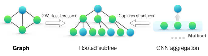
1-WL as Message Passing

The 1-WL iteration is exactly message passing with an injective aggregation. A general MPNN layer is

which is the 1-WL update with \(\mathrm{HASH}\) split into an aggregator and an update function. Setting \(\mathrm{AGG}\) to “collect the multiset” and \(\mathrm{UPDATE}\) to \(\mathrm{HASH}\) recovers colour refinement exactly. The requirement is that the composition be injective on multisets: distinct \(\bigl(h_v, \{\!\{h_u\}\!\}\bigr)\) must map to distinct outputs.

The Main Theorem (Xu et al., 2019)

Upper bound. Let \(G\) and \(G'\) be two graphs that 1-WL fails to separate. Then for any choice of message, aggregation and update functions, an MPNN produces the same multiset of node embeddings on \(G\) and \(G'\), and hence — after any permutation-invariant readout — the same graph-level embedding. Message-passing GNNs are therefore at most as expressive as 1-WL at distinguishing non-isomorphic graphs.

The proof is a straightforward induction on layers: if two nodes share a 1-WL colour at step \(k-1\), then their neighbour multisets of colours agree, so any function of those multisets returns the same value at step \(k\). An MPNN can only ever coarsen the 1-WL partition, never refine it.

Matching lower bound. Conversely, there exists an MPNN that is exactly as powerful as 1-WL — GIN. This direction is conditional, and the conditions matter:

• the node feature space must be countable, so that a multiset can be encoded injectively by a sum;
• the aggregator must be injective on multisets — sum qualifies, mean and max do not;
• the update MLP must be expressive enough to realise the required injective map (invoked via the universal approximation theorem).

Under those conditions the bound is tight: 1-WL is both a ceiling and an achievable target.

Two clarifications worth keeping straight:

• “At most as expressive as 1-WL” is a statement about distinguishing graphs, not about approximating functions or generalising from data. A GIN and a GCN separate exactly the same graph pairs in the ideal case, yet behave very differently in practice.
• The result says nothing about which graphs are hard. Almost all graphs are in fact identified by 1-WL; the failures are a structured, adversarial minority (regular graphs and their relatives) that happen to include chemically and combinatorially important cases.

Anything more expressive must leave the MPNN family altogether: higher-order WL, subgraph GNNs, graph Transformers, or structural/positional encodings.

What 1-WL Cannot Distinguish

Two classes of graphs that fool 1-WL (and therefore any MPNN). Both assume uniform initial node features — informative features can break these ties, which is why real molecular GNNs are not as helpless as the worst case suggests.

1. Regular graphs. If every node of \(G\) has degree \(k\), then all nodes get the same colour at every iteration and the colouring never refines. Consequently any two \(k\)-regular graphs on the same number of nodes produce identical 1-WL histograms, and no MPNN can separate them.

Triangle (3 nodes, 2-regular)  vs.  3 isolated nodes (0-regular)
  → distinguished: different degrees, hence different colours

Two non-isomorphic 3-regular graphs on 6 nodes
  → NOT distinguished by 1-WL, nor by any MPNN

2. Nodes with identical unrolled neighbourhoods. Two nodes \(v\) and \(v'\) receive the same colour after \(K\) iterations exactly when their unrolled computation trees to depth \(K\) coincide. Since a tree records no cycle structure, \(v\) can lie on a 4-cycle and \(v'\) not while both trees agree — so 1-WL cannot see the difference. Note the quantifier: this is about equality of the depth-\(K\) trees for the \(K\) actually run, and on regular graphs they agree for every \(K\).

GIN: The Most Expressive MPNN

GIN (Graph Isomorphism Network, Xu et al., 2019) achieves 1-WL expressiveness with the layer

where \(h^{(k)}_v\) is node \(v\)’s feature at layer \(k\), \(\mathcal{N}(v)\) its neighbourhood, and \(\varepsilon^{(k)}\) a scalar (fixed or learned) weighting a node’s own contribution against its neighbours’.

Sum aggregation (not mean or max) is what makes this work. Over multisets drawn from a countable universe, the sum of suitably encoded elements is injective; mean and max are not:

• Mean cannot distinguish \(\{\!\{1,1,1\}\!\}\) from \(\{\!\{1\}\!\}\) — it normalises away multiplicity
• Max cannot distinguish \(\{\!\{1,2,3\}\!\}\) from \(\{\!\{2,3\}\!\}\) — it discards everything but the extremum
• Sum separates both pairs: \(3 \ne 1\) and \(6 \ne 5\)

Two conditions are doing real work here and are often dropped when this result is quoted. The injectivity of the sum holds for multisets over a countable feature space (Xu et al. prove it by constructing an encoding whose sums are unique), and the \(\mathrm{MLP}\) must be expressive enough to realise the required injective map — invoked through universal approximation, which is an existence result, not something gradient descent is guaranteed to find.

Beyond 1-WL: Higher-Order Tests

To go beyond 1-WL, you need:

The \(k\)-WL hierarchy is strict: for \(k \ge 2\), \((k{+}1)\)-WL distinguishes strictly more graph pairs than \(k\)-WL. (The bottom of the hierarchy is the usual source of confusion — under the standard indexing, 1-WL and 2-WL have the same distinguishing power, and the first real gain comes at 3-WL.) The price is that \(k\)-WL colours \(k\)-tuples of nodes, so memory grows as \(N^{k}\).

Summary

The WL test is the lens through which GNN expressivity is understood. It tells you not just what GNNs can do, but precisely what they cannot — and why adding structural encodings, higher-order interactions, or global attention is necessary for harder graph reasoning tasks.

References

• Xu, K., Hu, W., Leskovec, J., & Jegelka, S. (2019). How Powerful are Graph Neural Networks?. ICLR 2019.
• Weisfeiler, B., & Lehman, A. A. (1968). A Reduction of a Graph to a Canonical Form and an Algebra Arising During This Reduction. Nauchno-Technicheskaya Informatsia.
• Babai, L., & Kucera, L. (1979). Canonical Labelling of Graphs in Linear Average Time. FOCS 1979.