
Audio-JEPA: Predicting Missing Sound Representations
Published:
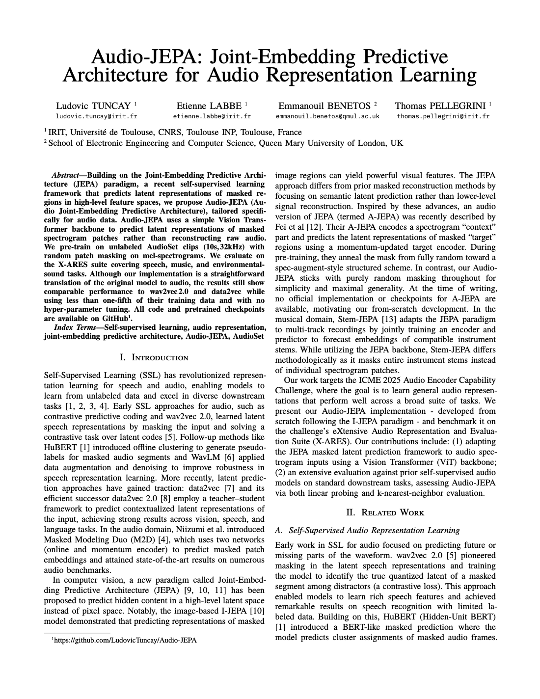
Ludovic Tuncay, Etienne Labbé, Emmanouil Benetos, and Thomas Pellegrini
Read the paper (PDF)
A spectrogram has two meaningful axes
Intuition first. A short recording of a door closing contains a sharp onset followed by decaying sound. A spectrogram displays how frequency content changes over time. Hiding some of its patches creates a prediction task in which nearby time and frequency structure can provide useful evidence.
Tuncay et al. adapt I-JEPA to mel-spectrograms using a vision-transformer backbone and random patch masking. This chapter covers their 2025 Audio-JEPA paper, which is distinct from the earlier A-JEPA: Joint-Embedding Predictive Architecture Can Listen by Fei et al.
The target is an embedding of the missing region
Let \(x\) denote spectrogram patches, \(M\) the masked indices, and \(\hat z_j\) the predictor output at a masked position. The objective is
The context branch receives visible patches; the target encoder processes the full spectrogram before the target positions are selected. Its parameters follow an exponential moving average of the context encoder. The predictor receives positional information for the missing patches. Paper, official implementation.
Worked example: count the prediction targets
Consider a \(128\times256\) spectrogram divided into \(16\times16\) patches. This gives
tokens. At an illustrative 50% masking ratio, the context encoder receives 64 visible tokens and the predictor is scored at 64 masked positions. The target encoder still sees the full spectrogram.
For a single target feature \((1,-1)\) and prediction \((0.8,-0.7)\), the squared feature error is \(0.2^2+0.3^2=0.13\). These coordinates are learned features, not amplitude samples or frequency values. A small feature loss therefore does not directly measure waveform reconstruction quality.
What frozen evaluation actually tests
The paper evaluates frozen representations with downstream classifiers and nearest-neighbour methods across audio tasks. A frozen encoder can still be paired with a classifier trained using labels. This protocol measures accessible task information, rather than an entire speech recognition or audio generation system. Evaluation setup.
Imagine two sounds recorded through the same microphone but describing different events. An encoder that mainly recognises the microphone can appear useful if recording devices correlate with labels. Splitting by recording source, when possible, tests whether the representation transfers beyond that shortcut.
A shared encoder still faces different task demands
Recognising an instrument may depend on timbre, whereas distinguishing similar spoken words may require fine temporal detail. One average benchmark score can hide this difference. Compare task families and inspect the effects of cropping, temporal resolution, and background noise.
Start with I-JEPA for the image formulation, then compare LLM-JEPA for a different way to use paired information in language training.
References
- Tuncay, L., Labbé, E., Benetos, E., & Pellegrini, T. Audio-JEPA: Joint-Embedding Predictive Architecture for Audio Representation Learning. 2025.
- Authors’ Audio-JEPA implementation.