
Diagonal, Orthogonal, and General Sheaf Maps
Published:
The Design Space of Restriction Maps
Intuition First: Think of the four map types as four different ways to describe the relationship between two people’s views of the same object. A scalar map says “person B sees things 3× more intensely than person A.” A diagonal map says “person B emphasises different colour channels differently.” An orthogonal map says “person B is looking from a rotated angle — same information, different frame.” A general map says “person B’s perception is a completely arbitrary linear combination of person A’s.” The richer the map class, the more relationships you can model — but the more parameters you need per edge.
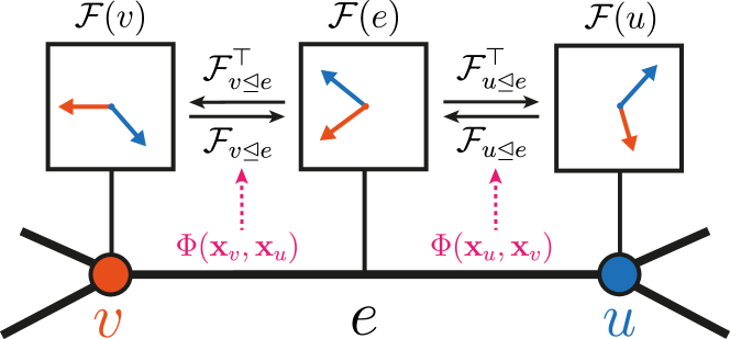
In Neural Sheaf Diffusion, the MLP outputs a restriction map F_{u→e} for each directed edge. The choice of matrix class constrains both what relationships the sheaf can represent and how much computation is required.
Scalar Maps (d_e = 1)
Parameters per edge: 1 (from the original d-dimensional node space to a 1-dimensional edge space).
What it represents: attention weight — how much of u’s contribution flows to edge e.
Sheaf Laplacian block: (Δ_F){uv} = -f{u→e} · f_{v→e} where f are scalars.
Connection to existing models: scalar sheaf maps recover GAT (graph attention network) with fixed attention weights.
Limitation: cannot represent directional transformations — just scaling.
Diagonal Maps
What it represents: per-dimension scaling — emphasise some feature dimensions over others.
Sheaf Laplacian block: (Δ_F)_{uv} = -diag(f_1^u f_1^v, …, f_d^u f_d^v). This is a diagonal matrix — the Sheaf Laplacian is block-diagonal in each feature dimension, so different dimensions are independent.
Advantage: O(d) parameters per edge (vs O(d²) for general); fast Sheaf Laplacian construction.
Limitation: cannot model inter-dimensional coupling — what node u thinks dimension 1 means is the same as what node v thinks dimension 1 means. Only magnitudes differ, not directions.
Orthogonal Maps
Parameters per edge: d(d-1)/2 (dimensions of the Lie group O(d)).
What it represents: rotations and reflections — a rigid transformation of feature space.
Key property: F^T_{u→e} F_{u→e} = I_d, so the diagonal block simplifies:
This means the diagonal blocks are scalar multiples of the identity — greatly simplifying the Sheaf Laplacian.
Connection geometry: orthogonal sheaves on graphs correspond exactly to flat vector bundles with orthogonal structure group — a classical object in differential geometry. This gives orthogonal sheaf GNNs a rich theoretical foundation connecting graph learning to Riemannian geometry.
General Linear Maps
Parameters per edge: d² (for square d×d maps) or d_e × d (for rectangular).
What it represents: arbitrary linear transformations — mixing, scaling, rotating, and projecting features.
Most expressive: can represent any linear relationship between u’s and v’s feature spaces.
Cost: O(d²) parameters per edge, O(d²) per Sheaf Laplacian block, O(E d²) total for the full Sheaf Laplacian.
Summary Comparison
| Map type | Parameters/edge | Feature coupling | Geometric meaning |
|---|---|---|---|
| Scalar | 1 | None | Attention weight |
| Diagonal | d | Per-dimension | Feature selection |
| Orthogonal | d(d-1)/2 | Full (rotation) | Frame rotation |
| General | d² | Full | Arbitrary linear |
Practical Recommendations
Use diagonal maps when: graphs are large (E » 1000), computation is a bottleneck, and per-dimension scaling is sufficient.
Use orthogonal maps when: geometry of the feature space matters (the maps should be interpretable as rotations), or when the theoretical connection to differential geometry is valuable.
Use general maps when: maximum expressiveness is needed and the graph is small enough (molecules, proteins with E < 10,000).
Impact on Sheaf Laplacian Sparsity
For all map types, the Sheaf Laplacian Δ_F has the same sparsity pattern as the standard graph Laplacian, but each scalar entry is replaced by a d×d block. The total size is (Nd) × (Nd) with at most 2E non-zero blocks (plus N diagonal blocks).
For diagonal maps, each block is diagonal — the Sheaf Laplacian is sparse in the d-expanded sense, enabling efficient sparse operations.
For general maps, each block is dense — the full Sheaf Laplacian requires O(E d²) storage.
References
- Bodnar, C., Giovanni, F. D., Chamberlain, B. P., Liò, P., & Bronstein, M. M. (2022). Neural Sheaf Diffusion: A Topological Perspective on Heterophily and Oversmoothing in GNNs. NeurIPS 2022 (NSD: compares scalar, diagonal, and general restriction map types, providing the theoretical and empirical analysis of each).
- Barbero, F., Bodnar, C., de Ocáriz Borde, H. S., Bronstein, M., Veličković, P., & Liò, P. (2022). Sheaf Attention Networks. NeurIPS 2022 Workshop (SheafAN: orthogonal restriction maps combined with attention, improving expressiveness and stability).
- Laplacian, H., & Curve, R. (2020). Orthogonal sheaf maps and connection Laplacians for robust graph learning. arXiv 2020 (theoretical analysis of orthogonal restriction maps and their connection to gauge-equivariant diffusion on graphs).