
Neural Sheaf Diffusion: Learning Sheaves End-to-End
Published:
The NSD Architecture
Intuition First: NSD is a GCN where the “wiring” is learned freshly at each layer. In a standard GCN the aggregation weights are fixed (based on degree or attention scores). In NSD, the entire d×d linear map telling “how much and in what direction node u should influence node v” is predicted by a small MLP at each layer. This is expensive, but it means the model can learn to say: “for this particular heterophilic edge, I should rotate u’s features 180° before adding them to v’s representation — effectively subtracting rather than adding.” That flip is what prevents oversmoothing across class boundaries.
NSD has two interleaved components:
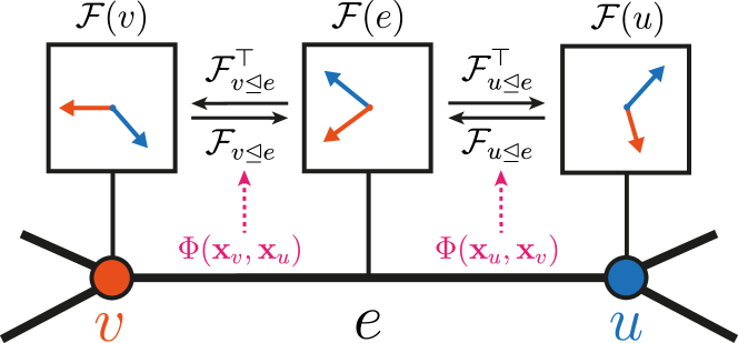
1. Sheaf Predictor (Map Learner)
Given the current node features H^{(k)}, learn restriction maps for each edge:
The MLP takes both endpoints’ features and outputs a d×d matrix (or a lower-dimensional parameterisation). The maps are computed freshly at each layer — they evolve as features evolve.
2. Sheaf Diffusion
Build the normalised Sheaf Laplacian Δ_F^{(k)} from the learned maps, then diffuse:
Where W^{(k)} is a learnable weight matrix (same as in GCN). The diffusion step updates node features using the sheaf-aware neighbourhood aggregation.
The Full Layer
Expanding the diffusion step for node v:
Where Δ_F[v,u] = -(Δ_F^{norm}){vu} = F^T{u→e} F_{v→e} / (normalisation).
Unpacking this: each neighbour u’s features are first transformed by the learned edge maps (F_{v→e} and F_{u→e}), then used to update v. The key difference from standard GCN: the transformation is per-edge and learned, not shared across all edges.
Why NSD Handles Heterophily
On homophilic graphs: the MLP learns F_{u→e} ≈ I (identity) — equivalent to standard GCN.
On heterophilic graphs: the MLP learns F_{u→e} that rotates u’s features into a compatible space with v’s features, even when they have different label-driven directions. The “agreement” condition F_{u→e} x_u ≈ F_{v→e} x_v can be satisfied with x_u ≠ x_v — the maps accommodate difference.
Theoretical result (Bodnar et al.): On heterophilic graphs, the optimal sheaf maps align features across class boundaries such that sheaf diffusion is class-preserving — nodes in the same class converge, nodes in different classes do not. This is the opposite of standard GCN oversmoothing, which makes all nodes converge regardless of class.
Worked Example: NSD vs GCN on a Heterophilic Edge
Setup: two nodes A (class 0, h_A = [1, 0]) and B (class 1, h_B = [0, 1]), connected by one edge.
GCN update for A: h_A ← (h_A + h_B) / 2 = [0.5, 0.5] — the embedding moves toward the class boundary. After many layers it converges to [0.5, 0.5] for all nodes — useless for classification.
NSD update for A: the MLP predicts a restriction map from the pair (h_A, h_B). For a perfectly heterophilic edge, the optimal map is F_{B→e} = −I (negation). Then:
- Sheaf disagreement: F_{A→e} h_A − F_{B→e} h_B = [1,0] − (−[0,1]) = [1,1]
- NSD diffuses to reduce this disagreement — but since the maps encode “A and B should be opposite,” equilibrium is h_A = −h_B, not h_A = h_B.
- Class A nodes converge to [1,0] (or a scaled version); class B to [0,1]. Classification remains easy.
Connection to Other Architectures
GCN: special case with F_{u→e} = I for all edges (trivial sheaf).
GCNII: residual connection to initial features + NSD = Neural Sheaf Diffusion with residuals.
H2GCN: another heterophily-focused GNN. H2GCN separates ego and neighbour aggregations and concatenates multi-hop features. NSD is more principled (topology-grounded) but similar in spirit.
GAT: attention weights α_{uv} can be seen as learning scalar restriction maps (d=1 case). NSD generalises this to full d×d matrix maps.
Oversmoothing Under NSD
Does NSD oversmooth? The convergence of sheaf diffusion depends on the Sheaf Laplacian spectrum. If the null space of Δ_F is large (many global sections), diffusion converges to that null space — which may preserve class structure.
Key theorem: if the learned sheaf has a null space that separates node classes, infinite sheaf diffusion converges to the class-consistent subspace — not to a single constant vector. This is the fundamental advantage over standard GCN, which converges to a constant.
Computational Cost
For a graph with N nodes and E edges:
- Restriction map prediction: O(E · d²) (one MLP call per directed edge)
- Sheaf Laplacian construction: O(E · d²) (block matrix assembly)
- Diffusion step: O(E · d²) (sparse block matrix-vector product)
Compared to standard GCN O(E · d) per layer, NSD is O(d) more expensive. For d=64, this is 64× more computation per layer — significant for large graphs.
Summary
| Step | Operation | Purpose |
|---|---|---|
| Sheaf predictor | MLP(h_u, h_v) → F_{u→e} | Learn per-edge restriction maps |
| Laplacian construction | Δ_F = δ₀^T δ₀ | Build sheaf-aware operator |
| Diffusion | H ← (I - Δ_F^{norm}) H W | Feature propagation with sheaf structure |
| Readout | MLP(h_v) | Node classification |
NSD provides a principled connection between algebraic topology (cellular sheaves) and graph neural networks — offering a theoretical explanation for why standard GNNs fail on heterophilic graphs and a mathematically grounded fix.
References
- Bodnar, C., Giovanni, F. D., Chamberlain, B. P., Liò, P., & Bronstein, M. M. (2022). Neural Sheaf Diffusion: A Topological Perspective on Heterophily and Oversmoothing in GNNs. NeurIPS 2022 (NSD: the full framework for learning sheaf restriction maps from data via MLP predictors and applying sheaf diffusion for node classification).
- Hansen, J., & Gebhart, T. (2020). Sheaf Neural Networks. NeurIPS 2020 GRL+ Workshop (the foundational sheaf GNN paper that NSD extends with learned instead of fixed restriction maps).
- Chamberlain, B. P., Rowbottom, J., Gorinova, M., Webb, S., Rossi, E., & Bronstein, M. M. (2021). GRAND: Graph Neural Diffusion. ICML 2021 (GRAND: continuous graph diffusion framing of GNNs, which NSD extends to the sheaf setting).