
Sheaf Neural Networks and Heterophily
Published:
The Heterophily Problem Revisited
Intuition First: On a heterophilic graph, running GCN is like trying to find your own position on a GPS by averaging all your neighbours’ coordinates, if you live at the boundary between two neighbourhoods, you will always end up placed in the wrong one. The sheaf solution is to give each boundary edge a “flip” map, so that crossing the boundary transforms features rather than blending them. The result is like placing a mirror at each class boundary: you see the reflection of the other side, not a blend.
Recall that in a heterophilic graph, nodes tend to connect to nodes of different classes. GCN’s aggregation is
with non-negative weights. When \(\mathcal{N}(v)\) contains mostly nodes of different classes, \(h_v\) becomes a mixture of other-class features, exactly wrong for node classification, where \(h_v\) should be discriminative for \(v\)’s own class.
What Happens to Standard GCN on Heterophilic Graphs
- Initial features \(x_v\) are (roughly) class-discriminative
- After one GCN layer, \(h_v\) is a weighted mean of different-class features and moves toward the inter-class centroid
- After more layers, \(h_v\) converges toward the dominant eigenvector of the propagation matrix, a single, class-independent profile
The reason is structural, not incidental. GCN’s propagation matrix is \(I - \tilde{\Delta}\) for the positively weighted graph Laplacian \(\tilde{\Delta}\), and the kernel of any such Laplacian on a connected graph is one-dimensional and constant. Diffusion converges to that kernel, so there is simply nowhere else for it to go. This is the catastrophic interaction between oversmoothing and heterophily.
The Sheaf Solution: Controlled Diffusion
With a learned sheaf \(\mathcal{F}\), diffusion minimises the sheaf Dirichlet energy
and converges to the set where it vanishes, namely \(\ker L_{\mathcal{F}} = H^0(G;\mathcal{F})\).
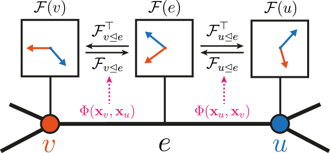
The key degree of freedom: the learned maps can make the transport \(\mathcal{F}_{v \trianglelefteq e}^{\top}\mathcal{F}_{u \trianglelefteq e}\) negative across a cross-class edge. Then “agreement” at that edge means \(x_v \approx -x_u\), and the class-discriminative signal is no longer penalised by the energy, it is a zero of it.
So the thing the sheaf’s extra structure buys is not a way of resisting diffusion. It is a way of changing where diffusion lands: \(\ker L_{\mathcal{F}}\) can be richer than the constant vectors, so the process does not have to collapse everything to one value.
There is a clean spectral way to see the same thing. On a bipartite graph the signed indicator \(v \mapsto \pm\sqrt{d_v}\) (positive on \(A\), negative on \(B\)) is the eigenvector of the normalised graph Laplacian for its largest eigenvalue \(\lambda = 2\), the highest possible frequency. Low-pass diffusion annihilates it fastest. A sheaf with the signs above moves that same signal to eigenvalue \(0\), where diffusion preserves it.
Comparison with Other Heterophily Methods
| Method | Heterophily strategy | Basis |
|---|---|---|
| GCN | Non-negative averaging (fails) | , |
| H2GCN | Separate ego/neighbour + multi-hop | Architectural heuristic |
| GPRGNN | Learnable polynomial filter | Spectral |
| FAGCN | Signed (low/high frequency) attention | Spectral, and a \(d=1\) sheaf in disguise |
| NSD (Sheaf) | Learned restriction maps + sheaf diffusion | Geometric / topological |
What distinguishes the sheaf framework is not that it is the only method with theory behind it, GPRGNN and FAGCN have spectral justifications too, but that it explains why signed and multi-frequency filters help, and generalises them: signed scalars are the \(d = 1\) case, and higher stalk dimensions extend the same argument to more than two classes.
Empirical Results
Accuracies on the two most-used heterophilic benchmarks, as reported in Bodnar et al. (2022), Table 1, on the ten fixed Geom-GCN splits (mean \(\pm\) std over splits; both datasets have five classes, so chance is 20%):
| Model | Chameleon (\(h = 0.23\)) | Squirrel (\(h = 0.22\)) |
|---|---|---|
| GCN | \(64.82 \pm 2.24\) | \(53.43 \pm 2.01\) |
| GAT | \(60.26 \pm 2.50\) | \(40.72 \pm 1.55\) |
| H2GCN | \(60.11 \pm 2.15\) | \(36.48 \pm 1.86\) |
| GPRGNN | \(46.58 \pm 1.71\) | \(31.61 \pm 1.24\) |
| Diag-NSD | \(68.68 \pm 1.73\) | \(54.78 \pm 1.81\) |
| \(O(d)\)-NSD | \(68.04 \pm 1.58\) | \(56.34 \pm 1.32\) |
| Gen-NSD | \(67.93 \pm 1.58\) | \(53.17 \pm 1.31\) |
Two things worth reading off this table. First, plain GCN is a strong baseline on these two datasets, the failure of standard message passing under heterophily is a matter of a few points, not a collapse to chance. Second, the general maps are not the winners: the diagonal and \(O(d)\) variants match or beat them, which is the empirical counterpart of the point made in the post on map types. More expressive is not automatically better.
(Chameleon and Squirrel are also known to contain many duplicated nodes; “filtered” versions of both are now commonly reported alongside the originals, and absolute numbers on the two versions are not comparable.)
Worked Example: Two-Class Bipartite Graph
Setup: the complete bipartite graph \(K_{2,2}\) with nodes \(A_1, A_2\) (class 0, features \([1,0]\)) and \(B_1, B_2\) (class 1, features \([0,1]\)). Every edge connects a class-\(A\) node to a class-\(B\) node.
Standard GCN. With self-loops every node has degree 3, so
Starting from \(x_A = [1,0]\), \(x_B = [0,1]\) the first layer gives \(x_A = [\tfrac13, \tfrac23]\) and \(x_B = [\tfrac23, \tfrac13]\). The discriminative difference obeys \(x_A - x_B \mapsto -\tfrac13 (x_A - x_B)\), so it shrinks by a factor of 3 per layer and both classes converge exponentially to \([0.5, 0.5]\). Classification becomes impossible.
NSD with well-chosen maps. Take stalks \(\mathbb{R}^2\) and set, on every edge,
The agreement condition at an edge \((A, B)\) is \(\mathcal{F}_{A \trianglelefteq e} x_A = \mathcal{F}_{B \trianglelefteq e} x_B\), i.e. \(x_A = R x_B\). With \(x_B = [0,1]\) we get \(R x_B = [1,0] = x_A\), they agree, in the sheaf’s sense, while being completely different vectors.
Because every \(A\)-node sees the same condition against every \(B\)-node, the harmonic space is
two-dimensional, and it contains the class-discriminative configuration. Diffusion converges to this space, so the class structure survives at equilibrium instead of being averaged away.
Why Sheaves Beat Heuristic Fixes
H2GCN separates the ego node from its neighbours and concatenates multi-hop features. This helps on many heterophilic graphs but is an architectural choice with no account of when it should work.
FAGCN uses signed attention (positive for same-class, negative for different-class). This is much closer in spirit to sheaf GNNs, in fact it is essentially the \(d = 1\) case, which explains both why it works on two-class heterophilic problems and why it runs out of room beyond them.
NSD provides a single framework that contains both: the restriction maps can represent identity (homophily), negation (anti-homophily), or any intermediate transformation, and the stalk dimension is the dial that extends the argument to many classes.
Summary
Sheaf GNNs address heterophily by replacing the implicit assumption of standard message passing (“neighbours should be equal”) with an explicit learned relationship per edge. Diffusion still converges to the kernel of its operator, but because that kernel can now be richer than the constant vectors, convergence no longer means collapse. This is the same fact viewed from two sides: it is why sheaf models resist oversmoothing, and why they help under heterophily.
References
- Bodnar, C., Di Giovanni, F., Chamberlain, B. P., Liò, P., & Bronstein, M. M. (2022). Neural Sheaf Diffusion: A Topological Perspective on Heterophily and Oversmoothing in GNNs. NeurIPS 2022 (the linear-separation results and the benchmark table quoted above).
- Zhu, J., Yan, Y., Zhao, L., Heimann, M., Akoglu, L., & Koutra, D. (2020). Beyond Homophily in Graph Neural Networks: Current Limitations and Effective Designs. NeurIPS 2020 (H2GCN; establishes the heterophily benchmark setting used above).
- Bo, D., Wang, X., Shi, C., & Shen, H. (2021). Beyond Low-frequency Information in Graph Convolutional Networks. AAAI 2021 (FAGCN: signed low/high-frequency attention, the \(d = 1\) sheaf in disguise).
- Lim, D., Li, X., Hohne, F., & Lim, S.-N. (2021). New Benchmarks for Learning on Non-Homophilous Graphs. arXiv 2021 (larger heterophily benchmark suite).