The Sheaf Laplacian: Spectral Theory for Sheaves

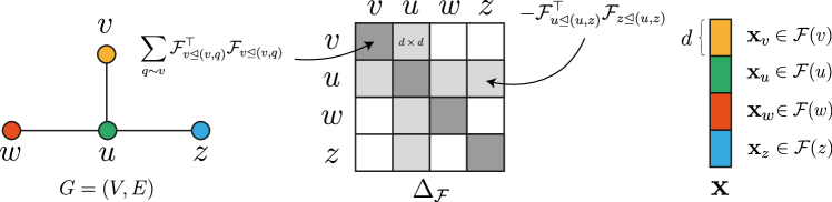
Constructing the Sheaf Laplacian

Intuition First: The standard graph Laplacian penalises adjacent nodes for being different (it minimises Σ (x_u − x_v)²). The Sheaf Laplacian instead penalises adjacent nodes for being inconsistent after transformation (it minimises Σ ‖F_{v→e} x_v − F_{u→e} x_u‖²). With identity maps, these are the same. With learned maps, “consistent” can mean “opposite in a structured way” — which is exactly what heterophilic graphs need.

Given a cellular sheaf F on graph G with coboundary map δ₀, the Sheaf Laplacian is:

Block structure: Δ_F is a block matrix indexed by nodes. For a graph with N nodes each having stalk ℝ^d, Δ_F ∈ ℝ^{Nd × Nd}. The blocks are:

Diagonal block for node v:

Off-diagonal block for edge e = (u,v):

Connection to the Standard Graph Laplacian

For the trivial sheaf (all F_{v→e} = I_d):

• Diagonal block: (Δ_F)_{vv} = deg(v) · I_d
• Off-diagonal block: (Δ_F)_{uv} = -I_d

This is exactly L ⊗ I_d = the Kronecker product of the standard graph Laplacian L with the identity — the multi-feature graph Laplacian. So the trivial sheaf recovers standard GCN.

Non-trivial restriction maps “twist” the off-diagonal blocks, changing how features from different nodes interact.

The Sheaf Dirichlet Energy

The quadratic form:

measures the total sheaf disagreement over the graph — how much the restriction maps disagree across all edges when applied to signal x.

• E_F(x) = 0 ↔ x is a global section (perfect consistency)
• E_F(x) is large ↔ x has large disagreement at many edges

Spectral view: eigenvectors of Δ_F with small eigenvalues correspond to signals with low sheaf Dirichlet energy — near-consistent signals. Diffusion with Δ_F drives signals toward global sections (null space of Δ_F).

Sheaf Diffusion

The heat equation on the sheaf:

Discretising with Euler step:

This is sheaf diffusion — the generalisation of GCN to sheaves. At each step, each node’s features are updated using the sheaf-weighted contributions of its neighbours.

For the normalised version, define the normalised Sheaf Laplacian:

Where D is the block-diagonal of Δ_F. The normalised diffusion H ← (I - Δ_F^{norm}) H is analogous to normalised GCN (Â = D^{-1/2} A D^{-1/2}).

Worked Example: 2-Node Sheaf Laplacian

Setup: two nodes u, v connected by one edge e. Stalks R^2. Restriction maps:

• F_{u→e} = [[1,0],[0,1]] (identity)
• F_{v→e} = [[0,1],[-1,0]] (90° rotation)

Diagonal block for u: (Δ_F){uu} = F{u→e}^T F_{u→e} = I

Diagonal block for v: (Δ_F){vv} = F{v→e}^T F_{v→e} = [[0,-1],[1,0]]^T [[0,1],[-1,0]] = I

Off-diagonal block: (Δ_F){uv} = −F{u→e}^T F_{v→e} = −[[0,1],[-1,0]]

Full 4×4 Sheaf Laplacian:

Δ_F = [[ 1,  0,  0, -1],
       [ 0,  1,  1,  0],
       [ 0, -1,  1,  0],
       [-1,  0,  0,  1]]

Global section (null space): Δ_F x = 0. From the equations: x_u = [[0,1],[-1,0]] x_v, which means x_v must satisfy R·x_v = x_v where R is a 90° rotation. No non-zero vector is fixed by 90° rotation, so the null space is trivial — no consistent global signal exists for this “twisted” sheaf.

Spectral Properties

Null space: Δ_F x = 0 ↔ δ₀ x = 0 ↔ x is a global section. The dimension of the null space (= number of zero eigenvalues) equals the number of linearly independent global sections.

For the trivial sheaf on a connected graph: null space has dimension d (one d-dimensional constant vector per component) — same as the standard graph Laplacian.

For a non-trivial sheaf: the null space can be larger or smaller. If the sheaf is “inconsistent” (no global sections beyond zero), the null space is trivial.

Spectral gap: the smallest non-zero eigenvalue of Δ_F determines how fast sheaf diffusion converges. Larger spectral gap → faster convergence → more aggressive feature mixing.

Normalised Sheaf Laplacian Spectrum

The eigenvalues of the normalised Sheaf Laplacian lie in [0, 2]:

• 0: global sections (consistent signals)
• Close to 0: nearly consistent signals
• Close to 2: maximally inconsistent signals

This is the same range as the standard normalised Laplacian. The difference: with non-trivial restriction maps, “consistency” is defined relative to the sheaf structure, not raw feature equality.

Summary

The Sheaf Laplacian is the central object for sheaf-based graph learning. It generalises the standard graph Laplacian by incorporating edge-level structure — making it possible to define diffusion that respects per-edge feature transformations rather than forcing raw feature equality.

References

• Hansen, J., & Gebhart, T. (2020). Sheaf Neural Networks. NeurIPS 2020 GRL+ Workshop (defines the Sheaf Laplacian Δ_F = δ₀^T δ₀ and Sheaf Dirichlet energy for graph learning; shows GCN is the scalar-sheaf special case).
• Bodnar, C., Giovanni, F. D., Chamberlain, B. P., Liò, P., & Bronstein, M. M. (2022). Neural Sheaf Diffusion: A Topological Perspective on Heterophily and Oversmoothing in GNNs. NeurIPS 2022 (NSD: analyses oversmoothing via the null space of Δ_F and shows learnable sheaf maps prevent convergence to trivial solutions).
• Ebli, S., Defferrard, M., & Spreemann, G. (2020). Simplicial Neural Networks. NeurIPS 2020 TDA & Beyond Workshop (related Hodge Laplacian approach on simplicial complexes, providing topological context for the Sheaf Laplacian).

References

- Hansen, J., & Ghrist, R. (2019). Toward a Spectral Theory of Cellular Sheaves. Journal of Applied and Computational Topology (defines \(L_{\mathcal{F}} = \delta^{\top}\delta\), its harmonic space, and the spectral bounds used above).