
What Is a Sheaf? From Topology to Graph Learning
Published:
Sheaves in Ordinary Mathematics
Intuition First: Imagine you’re assembling a jigsaw puzzle. Each piece (node) has part of the picture. Two adjacent pieces (connected by an edge) must agree along their shared border — but the border on piece A’s side is the same physical border as on piece B’s side, viewed from slightly different angles. The “restriction maps” are exactly the rotation/flip transforms that make A’s border match B’s border. A global section is a completed puzzle where every adjacent pair agrees perfectly after applying those transforms.
In mathematics, a sheaf is a tool for tracking local data (defined on open sets of a topological space) and understanding when local data can be assembled into global data.
The key property: local-to-global consistency. Data is consistent locally at every overlap → data assembles into a unique global section.
For our purposes (cellular sheaves on graphs), we use a discretisation: the “topological space” is the graph, “open sets” are nodes and edges, and “local data” are vectors in the stalks.
Cellular Sheaves on Graphs
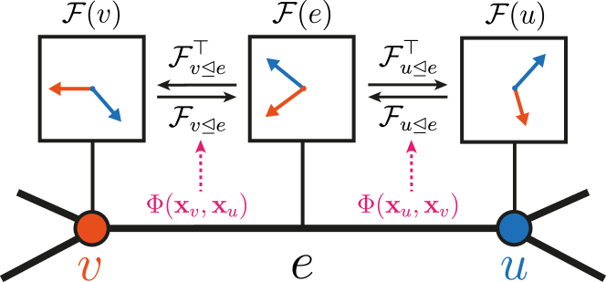
A cellular sheaf F on graph G = (V, E) assigns:
- Node stalks: a vector space F(v) = ℝ^{d_v} to each node v
- Edge stalks: a vector space F(e) = ℝ^{d_e} to each edge e
- Restriction maps: for each edge e = (u,v) and each incident node w ∈ {u,v}:
- F(w ⊴ e): F(w) → F(e) — a linear map from the node stalk to the edge stalk
Notation: F_{v→e} denotes the restriction map from node v to edge e.
The Cochain Complex
The stalks and restriction maps define a cochain complex:
Where:
- C^0 = ⊕_v F(v): the space of all node assignments (0-cochains)
- C^1 = ⊕_e F(e): the space of all edge assignments (1-cochains)
- δ₀: C^0 → C^1 is the coboundary map (codifferential):
The coboundary δ₀ x measures the disagreement between u’s and v’s contributions to edge e.
Global Sections
A global section is a vector x ∈ C^0 (assignment of vectors to all nodes) such that:
i.e., F_{v→e} x_v = F_{u→e} x_u for all edges e=(u,v). The two endpoints “agree” at every edge.
The space of global sections ker(δ₀) measures how much consistent global data the sheaf supports.
Special case — trivial sheaf: F(v) = ℝ, F(e) = ℝ, all restriction maps = 1. Then δ₀ x = x_v - x_u is just the ordinary graph gradient, and global sections are constant functions on connected components. This recovers the standard GCN setting.
The Standard Graph as a Trivial Sheaf
Standard GCN corresponds to the trivial sheaf:
- F(v) = ℝ^d for all v (all stalks the same space)
- F(e) = ℝ^d for all e
- F_{v→e} = I_d (identity map) for all v, e
The coboundary δ₀ x = x_v - x_u is just the edge-difference of features. The Sheaf Laplacian reduces to the standard graph Laplacian L = δ₀^T δ₀.
| GCN propagation H ← (I - L/2) H is graph diffusion — it minimises the Dirichlet energy Σ_{(u,v)} | x_u - x_v | ². |
Non-Trivial Sheaves Allow Disagreement
With non-trivial restriction maps, the “agreement” condition becomes F_{u→e} x_u = F_{v→e} x_v — x_u and x_v are not required to be equal, only to agree after transformation.
This allows adjacent nodes to have different but compatible features. In a heterophilic graph, two nodes with different labels might have very different features, but a learned sheaf map could rotate one into the other’s space — making them “consistent” under the sheaf even though they are numerically different.
Worked Example: Global Section on a Triangle Graph
Setup: triangle graph with nodes u, v, w. All stalks R^1 (scalars). Restriction maps: F_{u→e_uv}=1, F_{v→e_uv}=1, F_{v→e_vw}=2, F_{w→e_vw}=1, F_{u→e_uw}=1, F_{w→e_uw}=3.
Coboundary at edge e_uv: (δ₀ x){e_uv} = F{v→e_uv} x_v − F_{u→e_uv} x_u = x_v − x_u
Coboundary at edge e_vw: (δ₀ x){e_vw} = F{w→e_vw} x_w − F_{v→e_vw} x_v = x_w − 2 x_v
Global section condition (all coboundaries = 0):
- x_v − x_u = 0 → x_v = x_u
- x_w − 2 x_v = 0 → x_w = 2 x_u
- 3 x_w − x_u = 0 → 3(2 x_u) − x_u = 5 x_u = 0 → x_u = 0
Conclusion: the only global section is the zero vector — this sheaf has no non-trivial consistent signal. The non-trivial restriction maps made the three consistency constraints overdetermined.
Why Sheaves for Graphs?
The sheaf framework provides:
- Richer aggregation: edges have their own “mediation” structure (restriction maps)
- Heterophily handling: adjacent nodes with different features are not forced to agree — the restriction maps can accommodate difference
- Mathematical guarantees: the Sheaf Laplacian inherits spectral theory from the standard Laplacian, with richer structure
Interpretability: the consistency defect δ₀ x ² measures “how heterophilic” the data is under the learned sheaf
Summary
| Concept | Standard GCN | Cellular Sheaf |
|---|---|---|
| Node data | Vectors h_v ∈ ℝ^d | Vectors x_v ∈ F(v) = ℝ^{d_v} |
| Edge data | None | Vectors x_e ∈ F(e) = ℝ^{d_e} |
| Agreement condition | h_u = h_v at edges | F_{u→e} x_u = F_{v→e} x_v |
| Laplacian | L = D - A | Δ_F = δ₀^T δ₀ (Sheaf Laplacian) |
| Global sections | Constant functions | ker(δ₀): consistent assignments |
The sheaf framework generalises the standard graph to a richer structure that can encode per-edge relational information. The Sheaf Laplacian, covered in the next post, is the key operator that makes this actionable for graph learning.
References
- Hansen, J., & Gebhart, T. (2020). Sheaf Neural Networks. NeurIPS 2020 GRL+ Workshop (introduces cellular sheaves for graph learning; defines stalks, restriction maps, coboundary operator, and global sections in the GNN context).
- Bodnar, C., Giovanni, F. D., Chamberlain, B. P., Liò, P., & Bronstein, M. M. (2022). Neural Sheaf Diffusion: A Topological Perspective on Heterophily and Oversmoothing in GNNs. NeurIPS 2022 (NSD: learns sheaf restriction maps from node features, building on the cellular sheaf theory from Hansen & Gebhart).
- Curry, J. (2014). Sheaves, Cosheaves and Applications. PhD Thesis, University of Pennsylvania 2014 (mathematical foundation of cellular sheaf theory underlying sheaf neural networks).