Equivariant Sheaf Neural Networks

From Sheaves to Connections

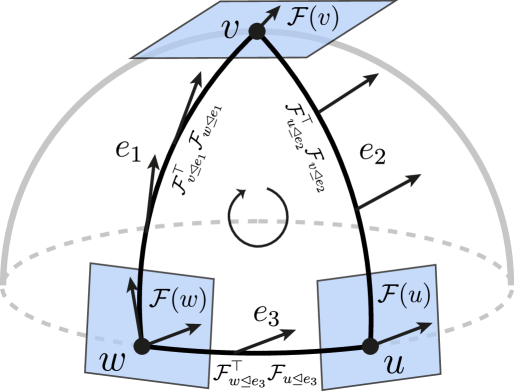
Intuition First: Imagine each node in the graph is a city with its own local coordinate system, “north” means something slightly different in New York than in Tokyo because the Earth is curved. To compare directions between cities you must transport a vector along a path between them, accounting for the curvature. That transport rule is the “connection.” In a sheaf with orthogonal maps, the edge maps are exactly this parallel transport: they tell you how to rotate a vector from node \(u\)’s local frame into node \(v\)’s. The “curvature” shows up when you go around a cycle and the transported vector has rotated away from where it started.

A cellular sheaf whose restriction maps are orthogonal, \(\mathcal{F}_{v \trianglelefteq e} \in O(d)\), is called a discrete \(O(d)\)-bundle. Each node carries a local frame, and the composite

transports a vector from \(u\)’s frame into \(v\)’s frame across the edge \(e\). Composing along a path \(\gamma\) gives \(P^{\gamma}_{v \to u}\), the transport along that path.

The holonomy around a cycle \(\gamma\) based at \(v\) is \(P^{\gamma}_{v \to v}\). If the transport is path-independent (all holonomies are the identity) the sheaf is flat, and the harmonic space is as large as it can be. In general Bodnar et al. show two complementary facts:

with \(\dim H^0 = d\) exactly when the transport is path-independent. Non-trivial holonomy shrinks the space of consistent global signals, it is the discrete analogue of curvature obstructing parallel sections.

The Connection Laplacian

For an \(O(d)\)-bundle the sheaf Laplacian takes a particularly clean form, and is then called the connection Laplacian:

The diagonal blocks collapse to degrees because \(\mathcal{F}^{\top}\mathcal{F} = I_d\), and each off-diagonal block is itself orthogonal.

Spectrum: the connection Laplacian is positive semi-definite. Because the diagonal blocks are \(\deg(v) I_d\) and the off-diagonal blocks have unit operator norm, Gershgorin gives eigenvalues in \([0,\, 2\deg_{\max}]\); after the normalisation \(\Delta_{\mathcal{F}} = D^{-1/2} L_{\mathcal{F}} D^{-1/2}\) they lie in \([0, 2]\), just as for the normalised graph Laplacian. Its kernel consists of the parallel sections, signals that are “constant” under parallel transport.

Gauge Symmetry

A gauge transformation is a choice of local frame change \(g_v \in O(d)\) at every node. It acts by

so that the value in the edge stalk, \(\mathcal{F}_{v \trianglelefteq e} x_v\), is unchanged. Writing \(g = \operatorname{blockdiag}(g_v)\), the Laplacian is conjugated:

The gauge-invariant quantities are those independent of the choice of local frames:

• the eigenvalues of \(L_{\mathcal{F}}\) (conjugation preserves the spectrum)
• edge disagreements \(\lVert \mathcal{F}_{v \trianglelefteq e} x_v - \mathcal{F}_{u \trianglelefteq e} x_u \rVert\), and hence the whole sheaf Dirichlet energy
• the conjugacy class of each holonomy \(P^{\gamma}_{v \to v}\), the holonomy matrix itself transforms as \(g_v P^{\gamma}_{v \to v} g_v^{-1}\), so it is its spectrum (e.g. the rotation angle) that is frame-independent, not its entries

A sheaf GNN should produce outputs that are gauge-invariant (for graph-level tasks) or gauge-equivariant (for node-level tasks, where the output lives in the node’s own frame).

Equivariant Sheaf GNN Layers

A gauge-equivariant layer must be built from quantities that transform predictably. At an edge \(e = (u,v)\):

Gauge-invariant:

• \(\lVert x_u \rVert\), \(\lVert x_v \rVert\)
• \(x_u^{\top} \mathcal{F}_{u \trianglelefteq e}^{\top} \mathcal{F}_{v \trianglelefteq e}\, x_v\), the inner product after transport
• \(\lVert \mathcal{F}_{v \trianglelefteq e} x_v - \mathcal{F}_{u \trianglelefteq e} x_u \rVert^2\), the edge’s contribution to the sheaf Dirichlet energy

Gauge-equivariant at \(v\) (i.e. transforming as \(g_v(\cdot)\)):

• \(P^{e}_{u \to v}\, x_u = \mathcal{F}_{v \trianglelefteq e}^{\top}\mathcal{F}_{u \trianglelefteq e}\, x_u\), neighbour \(u\)’s feature read in \(v\)’s frame

Note the index order: to land in \(v\)’s frame you transport from \(u\) to \(v\), so the transpose belongs to \(v\). Under a gauge transformation this becomes \((\mathcal{F}_{v} g_v^{-1})^{\top}(\mathcal{F}_{u} g_u^{-1})(g_u x_u) = g_v\,\mathcal{F}_{v}^{\top}\mathcal{F}_{u} x_u\), using \(g_v^{-\top} = g_v\) for orthogonal \(g_v\), the \(g_u\) cancels and only \(g_v\) survives, as required.

A complete equivariant sheaf layer therefore looks like

where \(\phi\) may be any map that is itself equivariant, for instance a linear combination, or an MLP applied to invariant scalars whose output rescales the equivariant vectors.

Connection to Equivariant GNNs for 3D Data

The geometric deep learning framework (EGNN, SE(3)-Transformers, TFN) handles \(E(n)\) / \(SE(3)\) equivariance for 3D point clouds. Sheaf GNNs with \(O(d)\) restriction maps handle \(O(d)\) gauge equivariance on abstract graphs. The structures are parallel but the groups act differently:

• 3D equivariant GNNs: one global rotation \(R \in SO(3)\) applied to the whole configuration
• Sheaf GNNs: an independent \(g_v \in O(d)\) at each node

Global equivariance is the special case \(g_v = g\) for all \(v\), the diagonal subgroup of the gauge group. Gauge equivariance is therefore the stronger requirement of the two: it constrains the model under a much larger group.

Applications

Point clouds with local frames: each point carries a local frame (surface normal plus tangent plane). Sheaf GNNs with orthogonal maps can process features in these frames and aggregate them consistently, the graph analogue of gauge-equivariant networks on meshes.

Protein structure: each residue has a local frame (the N–Cα–C backbone triad). The restriction maps encode how to transform between residue frames along the chain and across contacts.

Manifold-aware sheaf construction: rather than learning the maps end-to-end, one can compute orthogonal maps that optimally align the estimated tangent spaces of neighbouring data points under a manifold assumption, a geometrically motivated alternative that reduces both compute and overfitting.

Graph signal processing: the connection Laplacian generalises the graph Laplacian to vector-valued signals with local frame structure, and is the operator behind vector diffusion maps and angular synchronisation.

Summary

Equivariant sheaf GNNs sit at the intersection of algebraic topology, differential geometry, and graph learning, providing a principled framework for processing data with local frame structure on graphs.

References

• Bodnar, C., Di Giovanni, F., Chamberlain, B. P., Liò, P., & Bronstein, M. M. (2022). Neural Sheaf Diffusion: A Topological Perspective on Heterophily and Oversmoothing in GNNs. NeurIPS 2022 (discrete \(O(d)\)-bundles, path-dependent transport, and the bound \(\dim H^0 \le d\) quoted above).
• Barbero, F., Bodnar, C., Sáez de Ocáriz Borde, H., Bronstein, M., Veličković, P., & Liò, P. (2022). Sheaf Neural Networks with Connection Laplacians. ICML 2022 Workshop on Topology, Algebra, and Geometry in Machine Learning (builds orthogonal maps from a manifold assumption by aligning neighbouring tangent spaces, instead of learning them end-to-end).
• Hansen, J., & Ghrist, R. (2019). Toward a Spectral Theory of Cellular Sheaves. Journal of Applied and Computational Topology (spectral theory of sheaf Laplacians, including the orthogonal/connection case).
• Singer, A. (2011). Angular Synchronization by Eigenvectors and Semidefinite Programming. Applied and Computational Harmonic Analysis (recovering node frames from noisy relative rotations, the synchronisation problem that motivates connection Laplacians on graphs).
• Borgi, A., Severino, M., Silvestri, F., & Liò, P. (2026). Equivariant Sheaf Neural Networks: Learning Geometric Transport on Graphs. arXiv:2608.28853 (learns directed, matrix-valued transport between vector stalks under exact ambient \(E(n)\)-equivariance, with a completeness theorem for displacement-conditioned transport, covered in depth in this dedicated post).

References

- Bodnar, C., Giovanni, F. D., Chamberlain, B. P., Liò, P., & Bronstein, M. M. (2022). Neural Sheaf Diffusion: A Topological Perspective on Heterophily and Oversmoothing in GNNs. NeurIPS 2022 (NSD: introduces orthogonal restriction maps and their connection to O(d) gauge symmetry on graphs).