
Polynomial Neural Sheaf Diffusion
Published:
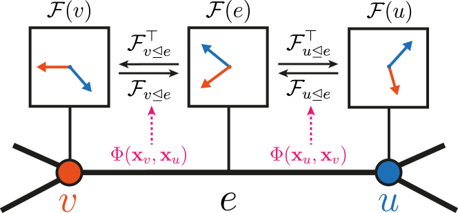
From Fixed Diffusion to Polynomial Filters
Intuition First: The fixed NSD filter \(h(\lambda) = 1 - \lambda\) is an audio equaliser with a single preset: bass boost, attenuating everything high. For homophilic graphs that is right, the class information lives in the smooth, low-frequency part of the signal. For heterophilic graphs you often want the opposite. PolyNSD gives you a programmable equaliser, learned from data: the \(K+1\) coefficients define the frequency response curve, and gradient descent picks the curve for the task.
NSD’s diffusion step (dropping the weights and non-linearity) is
a first-order polynomial in \(\Delta_{\mathcal{F}}\) with fixed coefficients. Spectrally it applies \(h(\lambda) = 1 - \lambda\) to each eigenvalue of \(\Delta_{\mathcal{F}} \in [0,2]\), a low-pass filter.
For homophilic graphs low-pass filtering is appropriate. For heterophilic graphs the class-discriminative content often sits at high \(\lambda\), where a fixed low-pass filter attenuates it. Note, though, that the sheaf already does part of this job: a learned sheaf can move a discriminative signal into the low-frequency end of \(\Delta_{\mathcal{F}}\)’s spectrum. The polynomial filter is the complementary lever, it decides what to do with the spectrum once the sheaf has shaped it.
The Polynomial Filter
Define the propagation operator as a degree-\(K\) polynomial:
Two design choices make this work in practice.
Spectral rescaling. Orthogonal polynomials are defined on \([-1,1]\), so the operator is rescaled first:
For the normalised sheaf Laplacian \(\lambda_{\max} = 2\) is known a priori, so the rescaling is simply \(\widetilde{\Delta}_{\mathcal{F}} = \Delta_{\mathcal{F}} - I\), no eigendecomposition and no power iteration needed.
Bounded coefficients. PolyNSD uses first-kind Chebyshev polynomials \(B_k = T_k\), which satisfy \(\lvert T_k(\xi) \rvert \le 1\) on \([-1,1]\), and parametrises the coefficients as a convex mixture, \(\theta = \operatorname{softmax}(\eta)\). Since \(\sum_k \theta_k = 1\) and \(\theta_k \ge 0\), the whole response satisfies \(\lvert p_\theta(\xi) \rvert \le 1\), the filter cannot blow up, whatever the network learns. Residual and gated paths around the filter supply the remaining flexibility. (The paper reports that other orthogonal bases, Legendre, Gegenbauer, Jacobi, perform comparably, so the stability comes from the construction rather than from Chebyshev specifically.)
Computing the Polynomial
Forming \(\Delta_{\mathcal{F}}^{k}\) explicitly would be hopeless: \(\Delta_{\mathcal{F}}\) is \(nd \times nd\) and its powers fill in. Chebyshev polynomials satisfy a three-term recurrence, so the filter is evaluated by repeated sparse products instead:
Each step is one sparse–dense product. A degree-\(K\) layer therefore costs \(O\big(K \cdot \mathrm{nnz}(\Delta_{\mathcal{F}}) \cdot f\big)\) for \(f\) feature channels, the same order as \(K\) stacked first-order sheaf layers, but with the sheaf predicted and the Laplacian assembled once instead of \(K\) times. That is where the practical speedup comes from: a \(K\)-hop receptive field in a single layer, decoupled from network depth.
The recurrence is also numerically better behaved than accumulating powers: because \(\lvert T_k \rvert \le 1\) on the rescaled spectrum, the intermediate \(Z^{(k)}\) do not grow.
Connection to Existing Methods
Polynomial filters unify a large part of the GNN literature. Writing \(\lambda\) for an eigenvalue of the relevant normalised Laplacian:
| Architecture | Filter \(h(\lambda)\) | Operator | Learnable? |
|---|---|---|---|
| GCN | \(1 - \lambda\) | Graph \(\Delta_0\) | Fixed, degree 1 |
| APPNP | \(\dfrac{\alpha}{1 - (1-\alpha)(1-\lambda)}\) | Graph \(\Delta_0\) | Fixed given \(\alpha\) (rational) |
| ChebNet | \(\sum_k \theta_k T_k(\lambda - 1)\) | Graph \(\Delta_0\) | Degree \(K\), learnable |
| GPRGNN | \(\sum_k \gamma_k (1-\lambda)^k\) | Graph \(\Delta_0\) | Degree \(K\), learnable |
| NSD | \(1 - \lambda\) | Sheaf \(\Delta_{\mathcal{F}}\) | Fixed, degree 1 |
| PolyNSD | \(\sum_k \theta_k T_k(\lambda - 1)\) | Sheaf \(\Delta_{\mathcal{F}}\) | Degree \(K\), learnable |
Read across the bottom two rows: PolyNSD is to NSD what ChebNet/GPRGNN are to GCN, with the crucial difference that the operator being filtered is a learned sheaf Laplacian rather than a fixed graph one.
Worked Example: Shaping the Frequency Response
Setup: normalised sheaf Laplacian with eigenvalues \(\lambda \in \{0,\ 0.5,\ 1.0,\ 1.5,\ 2.0\}\).
Fixed NSD filter, \(h(\lambda) = 1 - \lambda\):
| \(\lambda\) | 0 | 0.5 | 1.0 | 1.5 | 2.0 |
|---|---|---|---|---|---|
| \(h(\lambda)\) | 1.0 | 0.5 | 0.0 | −0.5 | −1.0 |
Magnitude decreases and then grows again with a sign flip; the “keep” region is the low end.
A degree-2 polynomial, \(h(\lambda) = \lambda^2 - 1\):
| \(\lambda\) | 0 | 0.5 | 1.0 | 1.5 | 2.0 |
|---|---|---|---|---|---|
| \(h(\lambda)\) | −1.0 | −0.75 | 0.0 | 1.25 | 3.0 |
Now the near-harmonic components are suppressed and the high-frequency ones amplified, a response the fixed degree-1 filter simply cannot produce, whatever scaling is applied to it. Note also that this particular \(h\) exceeds 1 in magnitude at \(\lambda = 2\); the softmax-over-Chebyshev parametrisation is precisely the device that rules such unbounded responses out while retaining the shape freedom.
Training and Practical Notes
- Degree \(K\): larger \(K\) means a longer receptive field and a more flexible response, at linear cost in sparse products. It is a receptive-field hyperparameter, not a depth one.
- Coefficients: shared across nodes and channels in the basic form. Making them node- or group-specific is possible but expensive.
- Restriction maps: notably, PolyNSD reports its strongest results using only diagonal restriction maps. This inverts the usual sheaf-GNN trend of pushing toward richer map classes and larger stalk dimensions: once the spectral response is learnable, the performance stops depending on a large \(d\), and the cheap map class is enough. Runtime and memory drop accordingly.
- Benchmarks: the paper reports state-of-the-art results across both homophilic and heterophilic node-classification datasets, including the “filtered” versions of Chameleon and Squirrel that remove duplicated nodes and on which many earlier numbers do not transfer.
Summary
| Property | NSD | PolyNSD |
|---|---|---|
| Sheaf maps | Learned | Learned (diagonal suffices) |
| Diffusion filter | Fixed, \(h(\lambda) = 1 - \lambda\) | Learnable degree-\(K\) polynomial |
| Spectral profile | Low-pass only | Learned response |
| Receptive field | 1 hop per layer | \(K\) hops per layer |
| Laplacian rebuilds | One per layer | One per layer, reused for all \(K\) terms |
| Extra parameters | None | \(K+1\) mixture logits per layer |
| Stability | Step-size dependent | Bounded by construction (\(\lvert p_\theta \rvert \le 1\)) |
PolyNSD combines the topological richness of cellular sheaves with the spectral flexibility of polynomial graph filters, addressing heterophily from both the structural and the spectral side at once, and, in doing so, removes much of the computational pressure that made earlier sheaf models expensive.
References
- Borgi, A., Silvestri, F., & Liò, P. (2025). Polynomial Neural Sheaf Diffusion: A Spectral Filtering Approach on Cellular Sheaves. arXiv:2512.00242 (PolyNSD: degree-\(K\) polynomial propagation on a normalised sheaf Laplacian, evaluated by a three-term recurrence on a spectrally rescaled operator, with a convex mixture of orthogonal-polynomial basis responses).
- Bodnar, C., Di Giovanni, F., Chamberlain, B. P., Liò, P., & Bronstein, M. M. (2022). Neural Sheaf Diffusion: A Topological Perspective on Heterophily and Oversmoothing in GNNs. NeurIPS 2022 (the base architecture that PolyNSD extends with a learnable polynomial diffusion filter).
- Defferrard, M., Bresson, X., & Vandergheynst, P. (2016). Convolutional Neural Networks on Graphs with Fast Localized Spectral Filtering. NeurIPS 2016 (ChebNet: the Chebyshev recurrence and spectral rescaling, on the ordinary graph Laplacian).
- Chien, E., Peng, J., Li, P., & Milenkovic, O. (2021). Adaptive Universal Generalized PageRank Graph Neural Network. ICLR 2021 (GPRGNN: learnable polynomial coefficients as the answer to heterophily on the ordinary graph Laplacian).
- He, M., Wei, Z., Huang, Z., & Xu, H. (2021). BernNet: Learning Arbitrary Graph Spectral Filters via Bernstein Approximation. NeurIPS 2021 (polynomial spectral filters in the Bernstein basis, with non-negativity constraints for stability).