
Equivariance: What It Means and Why It Matters
Published:
Groups and Symmetry
Intuition First: Think of a compass. No matter which direction you hold it, it still points north — the reading is invariant to how you rotate your body. Now think of your shadow: if you rotate 90°, your shadow rotates 90° too — the shadow is equivariant to your rotation. These two everyday observations capture the entire mathematical framework of geometric deep learning.
A group G is a set of transformations {g} with a composition rule, identity, and inverses. Symmetry groups relevant to 3D geometry:
- SE(3): rotations + translations in 3D (rigid body motions). SE = Special Euclidean.
- E(3): rotations + translations + reflections. E = Euclidean.
- E(n): rotations + translations + reflections in n-dimensional space.
- SO(3): rotations only (no reflections, no translations).
For molecular tasks: SE(3) or E(3) are the relevant groups.
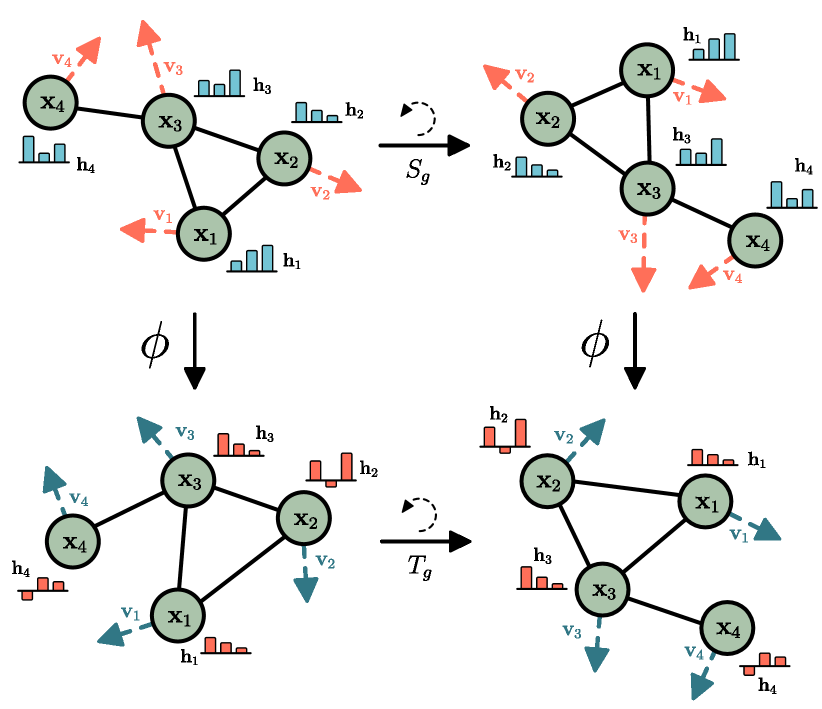
Invariance vs Equivariance
Let ρ_in and ρ_out be the representations of G on the input and output spaces respectively (i.e., how transformations act on inputs/outputs).
G-invariant: f(ρ_in(g) · x) = f(x). Output does not change when input is transformed.
Example: molecular potential energy. Rotating the molecule doesn’t change its energy.
G-equivariant: f(ρ_in(g) · x) = ρ_out(g) · f(x). Output transforms consistently with input.
Example: atomic forces. If we rotate the molecule, the forces rotate the same way.
Note: invariance is a special case of equivariance where ρ_out is the trivial representation (all g map to the identity).
Why Equivariance Is Better Than Augmentation
Data augmentation approach: train on random rotations of the molecule, hoping the model learns rotational invariance from data.
Problems:
- Requires many rotations per sample → expensive
- The model might learn approximate invariance, not exact invariance
- Generalisation to unseen orientations is not guaranteed
Equivariant approach: build the constraint into the architecture. The model is exactly equivariant by design — for any input orientation, the output transforms correctly. No augmentation needed.
Practical advantage: equivariant models achieve the same accuracy with ~10× fewer training samples than augmentation-based approaches on molecular benchmarks.
Worked Example: Invariant vs Equivariant in 2D
Setup: molecule with two atoms at positions r₁=(1,0) and r₂=(0,1). We apply a 90° counter-clockwise rotation R: (x,y)→(−y,x).
After rotation: r₁’=(0,1), r₂’=(−1,0).
Invariant quantity — distance:
- Before: ‖r₁−r₂‖ = ‖(1,−1)‖ = √2
- After: ‖r₁’−r₂’‖ = ‖(1,1)‖ = √2 ✓ same
Equivariant quantity — force vector (suppose F=(0.5, −0.5) before rotation):
- After rotation: R·F = (0.5, 0.5) ← force rotated by 90° too
- A model that outputs F=(0.5,−0.5) for the original and F=(0.5,0.5) for the rotated version is equivariant.
- A model that always outputs F=(0.5,−0.5) regardless of orientation is wrong — it breaks equivariance.
Representations: Scalars, Vectors, Tensors
The representation ρ_out determines how the output transforms:
Scalar (l=0 / invariant): a single number. Energy, charge, mass. Unchanged by rotation: ρ(R) = 1.
Vector (l=1 / equivariant): a 3D vector. Forces, velocities, dipole moment. Rotates with the molecule: ρ(R) = R.
Rank-2 tensor: a 3×3 matrix. Stress tensor, polarisability. Transforms as ρ(R) = R ⊗ R.
Irreducible representations (irreps) of SO(3): characterised by degree l. l=0 is scalar, l=1 is vector, l=2 is rank-2 tensor, etc. Higher l captures finer geometric information at increasing computational cost.
Types of Equivariant Models
Type 1: Distance-based invariance Features: only interatomic distances and angles. Output: scalar only. Architectures: SchNet, DimeNet. Limitation: cannot output vectors (forces require equivariant outputs).
Type 2: Vector-based equivariance (E(3)/SE(3)) Features: positions as vectors, combined with scalar features. Output: scalars + vectors. Architectures: EGNN, PaiNN, NequIP.
Type 3: Tensor field networks (full irreps) Features: spherical harmonics up to degree L. Output: arbitrary tensor fields. Architectures: TFN, SE(3)-Transformers, MACE. Limitation: expensive, O(L²) or O(L³) in degree.
Building Equivariant Layers
Any layer that combines inputs through:
- Equivariant linear maps (apply R consistently to all vectors)
- Invariant scalars (distances, norms)
- Tensor products (combining irreps)
is equivariant. The key constraint: never mix coordinates directly with scalars through arbitrary MLPs — that would break equivariance.
Summary
| Concept | Definition | Example |
|---|---|---|
| Invariant | f(Rx) = f(x) | Potential energy |
| Equivariant | f(Rx) = R f(x) | Forces |
| Augmentation | Learn symmetry from data | Expensive, approximate |
| Architectural equivariance | Baked-in symmetry | Exact, sample-efficient |
| Scalar (l=0) | Unchanged by rotation | Energy, charge |
| Vector (l=1) | Rotates with molecule | Force, velocity |
Equivariance is the mathematical foundation of geometric deep learning. Every architecture in the next posts — EGNN, SE(3)-Transformers, TFN — is a concrete instantiation of these principles.
References
- Bronstein, M. M., Bruna, J., Cohen, T., & Veličković, P. (2021). Geometric Deep Learning: Grids, Groups, Graphs, Geodesics, and Gauges. arXiv 2021 (comprehensive treatment of group symmetries, equivariance, and irreducible representations in deep learning).
- Cohen, T. S., & Welling, M. (2016). Group Equivariant Convolutional Networks. ICML 2016 (G-CNNs: first systematic framework for equivariant networks on discrete symmetry groups).
- Kondor, R., & Trivedi, S. (2018). On the Generalization of Equivariance and Convolution in Neural Networks to the Action of Compact Groups. ICML 2018 (theoretical foundation for equivariant neural networks over compact groups).