
EGNN: E(n)-Equivariant Graph Neural Networks
Published:
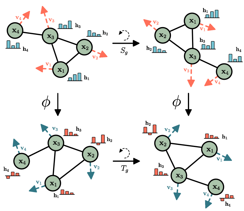
The EGNN Approach
Intuition First: EGNN is like a choreography that works in any room orientation. Each dancer (atom) tracks two things: their personal identity (invariant features \(h_i\), atomic number, charge) and their position on stage (equivariant coordinates \(x_i\)). When two dancers communicate, they whisper only about the distance between them (invariant), then each adjusts their stage position by moving slightly toward or away from the other. Because they only use relative positions, never absolute coordinates, the whole dance looks the same whether the room is rotated 30° or 300°.
EGNN maintains two quantities per node:
- \(h_i \in \mathbb{R}^d\): invariant features
- \(x_i \in \mathbb{R}^n\): equivariant coordinates (\(n = 3\) for 3D)
These are updated jointly across layers, always maintaining \(\mathrm{E}(n)\) equivariance.
The EGNN Update Rule
Edge messages (invariant quantities only):
The message uses the squared distance \(\lVert x_i - x_j \rVert^2\), an \(\mathrm{E}(n)\)-invariant scalar. The optional edge attribute \(a_{ij}\) is invariant too. Squared rather than plain distance only to avoid the square root’s non-differentiability at zero; nothing about the symmetry argument depends on the choice.
Coordinate update (equivariant):
Crucially \(\phi_x : \mathbb{R}^{d} \to \mathbb{R}\) outputs a scalar. The direction of each contribution comes entirely from the relative vector \((x_i - x_j)\); the network only decides how far to move along it, never where to point.
Feature update (invariant):
Features are updated only from invariant messages, so \(h_i\) stays invariant.
Why This Is Automatically E(n)-Equivariant
The argument is short enough to give in full, and it is worth doing because it shows why no spherical harmonics are needed. Apply \(x_i \mapsto Q x_i + t\) for any orthogonal \(Q\) and any translation \(t\).
Step 1, the messages don’t move. The translation cancels in the difference and the rotation cancels in the norm:
So \(m_{ij}\) is unchanged, hence so are \(\phi_x(m_{ij})\) and every \(h_i\). The feature stream is invariant.
Step 2, the coordinates carry the transformation through. Since the scalars \(\phi_x(m_{ij})\) are now known to be unchanged, they pull straight out of the linear map:
which is exactly \(Q x_i^{\text{new}} + t\). Transforming the input and then running the layer gives the same answer as running the layer and then transforming the output.
Two things to notice about the conditions. First, the only property of \(Q\) used is \(Q^{\!\top}Q = I\), nothing required \(\det Q = +1\). The equivariance therefore holds for the full \(\mathrm{E}(n)\), reflections included, not merely \(\mathrm{SE}(n)\). Second, that is a genuine limitation as well as a feature: an \(\mathrm{E}(n)\)-equivariant network gives mirror-image inputs mirror-image outputs and mirror-image scalars that are identical, so plain EGNN cannot distinguish enantiomers. If chirality matters, you need reflection-odd features that EGNN does not have.
Comparison to TFN / SE(3)-Transformers
| Property | EGNN | TFN / SE(3)-Trans |
|---|---|---|
| Symmetry group | \(\mathrm{E}(n)\) | \(\mathrm{SE}(3)\) (with parity bookkeeping, \(\mathrm{E}(3)\)) |
| Geometric features | Distances + relative positions | Spherical harmonics (irreps) |
| Cost per edge | \(O(d)\), one MLP | Grows steeply with max degree \(L\) (many CG paths, each contracting irreps of size up to \(2L+1\)) |
| Output types | Scalars and vectors (\(\ell \le 1\)) | Any degree \(\ell \le L\) |
| Machinery | Plain MLPs | Clebsch–Gordan tensor products |
| Chirality | Blind to it (reflection-equivariant) | Can be made sensitive via parity |
EGNN gives up representations beyond \(\ell = 1\), no \(\ell = 2\) or higher outputs, in exchange for dramatically simpler and faster computation.
Applications
Molecular dynamics: predict energies and forces. Forces are the negative gradient of the energy, and the gradient of an invariant scalar is an equivariant vector, so differentiating an invariant energy head gives equivariant forces for free.
N-body simulation: predict trajectories of charged particles. EGNN models the interaction forces and propagates positions forward.
Protein structure: predict residue positions given contact maps. Equivariance ensures predictions rotate consistently with the input.
Point cloud processing: EGNN applied to LiDAR point clouds maintains rotational equivariance for 3D object detection, with the caveat that for scenes with a fixed gravity direction, full rotational equivariance is a stronger constraint than the data actually requires.
Worked Example: One EGNN Layer on 3 Atoms
Setup: 3 atoms, H at \(x_1 = (0,0,0)\), O at \(x_2 = (1,0,0)\), H at \(x_3 = (1,1,0)\). Features \(h_1 = h_3 = 1\) (hydrogen), \(h_2 = 2\) (oxygen). Take \(\phi_e\) and \(\phi_x\) to be simple fixed functions for illustration.
Step 1, Edge messages (squared distances):
- H–O edge: \(m_{12} = \phi_e(h_1, h_2, \lVert x_1 - x_2 \rVert^2) = \phi_e(1, 2, 1.0)\)
- O–H edge: \(m_{23} = \phi_e(h_2, h_3, \lVert x_2 - x_3 \rVert^2) = \phi_e(2, 1, 1.0)\)
- H–H pair: \(m_{13} = \phi_e(h_1, h_3, \lVert x_1 - x_3 \rVert^2) = \phi_e(1, 1, 2.0)\), the longer, non-bonded pair
Step 2, Coordinate update for O (atom 2), taking \(C = 1\):
- Update rule: \(x_2 \leftarrow x_2 + (x_2 - x_1)\,\phi_x(m_{12}) + (x_2 - x_3)\,\phi_x(m_{23})\)
- Relative vectors: \((x_2 - x_1) = (1,0,0)\) and \((x_2 - x_3) = (0,-1,0)\)
- With \(\phi_x = 0.1\) on both edges: \(x_2 \leftarrow (1,0,0) + 0.1(1,0,0) + 0.1(0,-1,0) = (1.1,\, -0.1,\, 0)\)
Equivariance check. Rotate everything by 90° about the \(z\)-axis, \(Q : (a,b,c) \mapsto (-b, a, c)\). Then \(x_1 \to (0,0,0)\), \(x_2 \to (0,1,0)\), \(x_3 \to (-1,1,0)\).
The squared distances are unchanged (\(1.0\), \(1.0\), \(2.0\)), so \(\phi_x\) still returns \(0.1\) on both edges, this is the step that makes the rest work. Then:
- Relative vectors: \((x_2' - x_1') = (0,1,0)\) and \((x_2' - x_3') = (1,0,0)\)
- Updated position: \(x_2' \leftarrow (0,1,0) + 0.1(0,1,0) + 0.1(1,0,0) = (0.1,\, 1.1,\, 0)\)
And \(Q\,(1.1, -0.1, 0) = (0.1, 1.1, 0)\) ✓, the updated coordinate is exactly the rotation of the update computed in the original frame. The same computation with a reflection in place of the rotation also goes through, which is precisely why the guarantee is \(\mathrm{E}(n)\) rather than \(\mathrm{SE}(n)\).
EGNN vs SchNet
SchNet (Schütt et al., 2017) is an earlier distance-based model: messages depend on \(\lVert x_i - x_j \rVert\), so it is \(\mathrm{E}(3)\)-invariant. But SchNet does not update coordinates, it only updates scalar features, so it can output energies and not forces directly. EGNN updates both features and coordinates, so it has an equivariant output stream and can predict vector quantities (forces, displacements) directly.
Training EGNN
For energy prediction:
- Target: energy \(E\) (scalar), use an invariant readout \(E = \sum_i \phi_{\text{out}}(h_i)\), which is invariant because every \(h_i\) is
- Loss: \(\mathrm{MSE}(E_{\text{pred}}, E_{\text{true}})\)
For force prediction, two options:
- Conservative: \(F_i = -\,\partial E / \partial x_i\) by autograd. Because \(E\) is invariant, its gradient with respect to coordinates is automatically equivariant, and the resulting force field is conservative by construction, energy is conserved along a simulated trajectory.
- Direct: predict \(F_i\) with an equivariant output head. Cheaper (no second derivative during training) but the predicted field is not guaranteed to be the gradient of any scalar, so it need not conserve energy in long molecular dynamics rollouts.
Training on energies and forces jointly improves generalisation, forces are the gradient of the target surface, so each force label carries far more information about it than an energy label does.
Summary
| Component | Behaviour under \(x \mapsto Qx + t\) | Why |
|---|---|---|
| \(m_{ij}\) (messages) | Invariant | Built from \(\lVert x_i - x_j \rVert^2\) only |
| \(x_i\) update | Equivariant | Scalar-weighted sum of \((x_i - x_j)\) |
| \(h_i\) update | Invariant | Consumes only invariant messages |
| Graph readout | Invariant | Sum of invariant node features |
| Reflections | Included | The proof needs only \(Q^{\!\top}Q = I\) |
EGNN is the practical choice when \(\mathrm{E}(n)\) equivariance is needed and the task requires only scalar (energy) or vector (force) outputs. For higher-degree outputs, or for anything reflection-sensitive, TFN, MACE or a parity-aware model is needed instead.
References
- Satorras, V. G., Hoogeboom, E., & Welling, M. (2021). E(n) Equivariant Graph Neural Networks. ICML 2021 (EGNN: E(n)-equivariant message passing using only interatomic distances, no spherical harmonics required).
- Schütt, K. T., Kindermans, P.-J., Sauceda Felix, H. E., Chmiela, S., Tkatchenko, A., & Müller, K.-R. (2017). SchNet: A Continuous-Filter Convolutional Neural Network for Modeling Quantum Interactions. NeurIPS 2017 (SchNet: the simpler predecessor using only distances, motivating EGNN’s invariant message design).
- Hoogeboom, E., Satorras, V. G., Vignac, C., & Welling, M. (2022). Equivariant Diffusion for Molecule Generation in 3D. ICML 2022 (EDM: applying EGNN equivariance to 3D molecule generation via diffusion models).