
MPNN: The General Message Passing Neural Network Framework
Published:
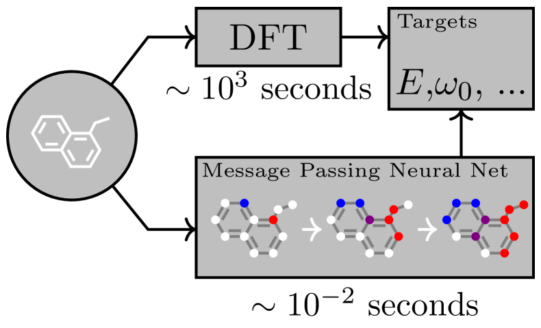
Intuition First: What Is Message Passing?
Imagine a group of friends, each holding a colored card. In each round, everyone passes their card color to their neighbors, who blend the incoming colors with their own. After K rounds, each person’s card encodes a summary of their K-hop social circle. That is message passing: iterative local information exchange that builds up increasingly global representations.
Why a Unified Framework?
By 2017, several successful GNN architectures existed, GCN, GGNN (Gated Graph Neural Network), Interaction Networks, etc. Each was described differently, making comparison and design difficult.
Gilmer et al. (2017) introduced MPNN to unify all spatial GNNs under one abstraction. This framework:
- Makes design choices explicit and comparable
- Enables systematic ablation and design
- Identifies what is shared and what differs between architectures
- Reveals the fundamental limits of the class (later formalised by the WL test)
The MPNN Framework
A single MPNN layer for node \(v\) computes three phases. Throughout, \(h_v^{(k)}\) is the state of node \(v\) after round \(k\) (with \(h_v^{(0)}\) the input features), \(\mathcal{N}(v)\) is the neighbourhood of \(v\), and \(e_{uv}\) is the feature vector of the edge between \(u\) and \(v\).
Phase 1, Message Computation:
For each neighbour \(u\) of \(v\), compute a message. The message function \(M^{(k)}\) can depend on the sender’s state \(h_u\), the receiver’s state \(h_v\), and the edge feature \(e_{uv}\).
Phase 2, Aggregation:
Aggregate all messages from neighbours. The operator \(\square\) must be permutation-invariant, the order of neighbours must not matter, because \(\mathcal{N}(v)\) is a set, not a sequence. Usual choices: sum, mean, max; an LSTM only qualifies approximately, by being fed a random permutation of the neighbours.
Phase 3, Update:
Combine the aggregated message with the node’s previous state to produce the new state.
After \(K\) rounds, each node’s representation \(h^{(K)}_v\) encodes information from its \(K\)-hop neighbourhood.
Concrete Worked Example: One MPNN Step
Consider a tiny graph: nodes A, B, C where A–B and B–C are edges. All nodes have scalar features, \(h_A = 1\), \(h_B = 2\), \(h_C = 3\). Take the simplest possible instance, identity message \(M(h_v, h_u, e_{uv}) = h_u\), mean aggregation, and update \(U(h_v, m_v) = \operatorname{ReLU}(h_v + m_v)\):
Step for node B (neighbours: A and C):
- Message from A: \(m_{A \to B} = h_A = 1\)
- Message from C: \(m_{C \to B} = h_C = 3\)
- Aggregation: \(m_B = \operatorname{mean}(1, 3) = 2.0\)
- Update: \(h_B' = \operatorname{ReLU}(h_B + m_B) = \operatorname{ReLU}(2 + 2) = 4\)
Step for node A (neighbour: B only):
- Message from B: \(m_{B \to A} = h_B = 2\)
- Aggregation: \(m_A = 2.0\)
- Update: \(h_A' = \operatorname{ReLU}(1 + 2) = 3\)
After one step, \(h_A\) has absorbed B’s information and \(h_B\) has blended A and C. After two steps, \(h_A\) would know about C, its 2-hop neighbour.
Popular GNNs as MPNN Instances
Here \(\tilde{d}_u\) is the degree of \(u\) in \(\tilde{A} = A + I\), \(\alpha_{vu}\) is a GAT attention coefficient, and \(\Vert\) is concatenation.
| Model | Message \(M\) | Aggregation \(\square\) | Update \(U\) |
|---|---|---|---|
| GCN | \(\dfrac{h_u}{\sqrt{\tilde{d}_u \tilde{d}_v}}\) | Sum (over \(\mathcal{N}(v) \cup \{v\}\)) | \(\sigma(W m_v)\) |
| GraphSAGE | \(h_u\) | Mean (or max-pool) | \(\sigma\big(W [\, h_v \Vert m_v \,]\big)\) |
| GAT | \(\alpha_{vu} W h_u\) | Sum | \(\sigma(m_v)\) |
| GIN | \(h_u\) | Sum | \(\operatorname{MLP}\big((1+\epsilon) h_v + m_v\big)\) |
| MPNN (original) | \(\mathcal{E}(e_{uv}) \, h_u\) | Sum | \(\operatorname{GRU}(h_v, m_v)\) |
Where \(\mathcal{E}(\cdot)\) is a learned edge network and GRU is a gated recurrent unit.
Edge Features in MPNN
A key advantage of the MPNN formulation: edge features are first-class citizens. The message function \(M\) can freely use \(e_{uv}\):
Here \(\mathcal{E}(e_{uv})\) is a matrix produced from the edge feature by a small learned network, the “edge network” of Gilmer et al., so each bond type induces its own linear map. This is essential for molecules, where bond types (single, double, aromatic) are critical features.
Readout for Graph-Level Prediction
After \(K\) message-passing rounds, MPNN computes a graph-level representation via a readout function:
The readout \(R\) must also be permutation-invariant, since \(V\) carries no canonical ordering. Common choices:
- Sum: \(h_G = \sum_{v \in V} h_v^{(K)}\), retains graph size
- Mean: \(h_G = \frac{1}{\lvert V \rvert} \sum_{v \in V} h_v^{(K)}\), size-invariant
- Set2Set: an attention-based readout with memory, used in the original MPNN paper
The Limits of MPNN
All MPNN models share the same fundamental limitation: their expressive power is bounded by the 1-dimensional Weisfeiler-Leman graph isomorphism test (1-WL; see the GIN post for the proof and the architecture that attains the bound).
Any two graphs that 1-WL cannot distinguish are also indistinguishable by any MPNN. If two nodes have the same multiset of neighbour features at every hop, no choice of \(M\), \(\square\) and \(U\) will separate them.
This limitation motivates:
- Higher-order GNNs (k-WL for k > 1)
- Structural encodings (adding positional/structural features that break symmetry)
- Graph Transformers (attend globally, not just to neighbours)
Practical Implementation
In PyTorch Geometric, MPNN-style models are implemented by inheriting MessagePassing:
class MyGNNLayer(MessagePassing):
    def __init__(self):
        super().__init__(aggr='sum')  # □ = sum

    def forward(self, x, edge_index, edge_attr):
        return self.propagate(edge_index, x=x, edge_attr=edge_attr)

    def message(self, x_j, edge_attr):
        # M: message from j to i
        return self.edge_net(edge_attr) @ x_j.unsqueeze(-1)

    def update(self, aggr_out, x):
        # U: update node state
        return self.gru(aggr_out, x)
Summary
The MPNN framework captures every spatial GNN in three functions:
| Function | Role | Must satisfy |
|---|---|---|
| \(M\) (message) | Compute edge messages \(m_{u \to v}\) | Can use sender, receiver and edge features |
| \(\square\) (aggregation) | Combine neighbour messages into \(m_v\) | Permutation-invariant |
| \(U\) (update) | Update node state | Combines old state \(h_v\) with the aggregate \(m_v\) |
The space of MPNNs is defined by the choices of \(M\), \(\square\) and \(U\). Understanding this space, and its limits, is the foundation for understanding all GNN research from 2016 to the present.
References
- Gilmer, J., Schoenholz, S. S., Riley, P. F., Vinyals, O., & Dahl, G. E. (2017). Neural Message Passing for Quantum Chemistry. ICML 2017.
- Veličković, P., Cucurull, G., Casanova, A., Romero, A., Liò, P., & Bengio, Y. (2018). Graph Attention Networks. ICLR 2018.
- Hamilton, W. L., Ying, R., & Leskovec, J. (2017). Inductive Representation Learning on Large Graphs. NeurIPS 2017.