Temporal Graph Networks: Learning from Events

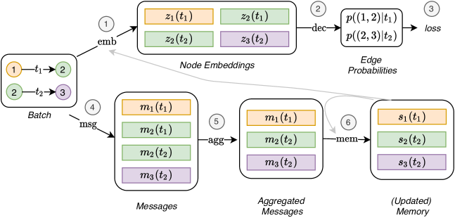
TGN’s Design Philosophy

TGN separates two concerns:

1. Memory: long-term history of a node’s interactions, stored as a fixed-size vector s_v
2. Embedding: current structural context, computed by aggregating recent neighbours

This separation allows efficient online updates (only memory changes on each event) while preserving rich structural context when embeddings are needed.

The TGN Components

1. Memory Module

Each node v has a memory state s_v ∈ ℝ^{d_s}. Initially s_v = 0.

When an interaction (u, v, t, e_{uv}) occurs:

• Node u interacts with node v at time t with edge features e_{uv}

Raw messages are computed for both interacting nodes:

Where s_u(t^-) is u’s memory just before the event, and Δt = t - t_last_u is the time since u’s last interaction.

Memory update (GRU):

The GRU’s gating mechanism naturally handles the trade-off between old memory and new information.

2. Temporal Graph Attention (Embedding Module)

When we need node u’s embedding at time t (for inference), we aggregate from temporal neighbours:

Time encoding: encode elapsed time as a feature using random Fourier features or learnable frequencies:

This gives the model a sense of recency — events further in the past have lower encoded similarity to the current time.

Temporal attention over neighbours:

Where N_k(u, t) is the k most recent temporal neighbours of u before time t.

3. Link Prediction Decoder

Given node embeddings h_u(t) and h_v(t), compute interaction probability:

Trained with binary cross-entropy + negative sampling (sample random non-interacting pairs as negatives).

Worked Example: One TGN Memory Update

Suppose user u has memory s_u = [0.5, -0.2, 0.8] (d_s = 3). At time t=100, u interacts with item v (s_v = [0.1, 0.9, 0.3]) via edge features e_uv = [1] (e.g., a “click”). The time since u’s last interaction: delta_t = 100 - 85 = 15.

Step 1: Raw message for u

m_u = MSG_s(s_u, s_v, delta_t, e_uv)
    = Linear([s_u || s_v || delta_t || e_uv])
    = Linear([0.5, -0.2, 0.8,  0.1, 0.9, 0.3,  15,  1])
    → suppose m_u = [0.3, 0.7, -0.1]   (after linear + activation)

Step 2: GRU memory update

s_u(t=100) = GRU(m_u, s_u(t^-))
           = GRU([0.3, 0.7, -0.1],  [0.5, -0.2, 0.8])
           → suppose s_u = [0.45, 0.6, 0.3]   (gate blends old + new)

The GRU’s forget gate suppresses the old memory dimension 3 (0.8 → 0.3) because the new message strongly activates it differently. Dimension 2 rises (−0.2 → 0.6) reflecting the new interaction. This is all differentiable — gradients flow back through the GRU to learn what to remember.

The Full TGN Loop

For each event (u, v, t, e_{uv}) in the stream:
  1. Retrieve memories s_u(t^-), s_v(t^-)
  2. Compute messages m_u, m_v
  3. Update memories: s_u(t), s_v(t)
  4. When evaluation needed:
     a. Compute temporal embeddings h_u(t), h_v(t)
     b. Predict p(u, v, t)

Variants and Ablations

TGN subsumes several prior architectures:

TGN-attn (full TGN) outperforms all ablations on link prediction benchmarks (Wikipedia, Reddit, MOOC, LastFM).

Inductive Capability

TGN naturally handles new nodes: when a previously unseen node v appears, its memory is initialised to 0. After its first few interactions, the memory accumulates history. This is the key advantage over transductive methods that require all nodes at training time.

Batch Processing and Training

Online event processing is not directly compatible with batched GPU training. TGN uses a trick: process events in chronological order within batches, carrying memory states forward. Memory updates are detached from the computation graph to avoid BPTT over the full event history — only the embedding computation and the final prediction are differentiated.

Summary

TGN is the standard baseline for continuous-time dynamic graph link prediction. Its modular design (memory + embedding + decoder) allows ablation studies and component swapping — making it a useful research framework as well as a practical model.

References

• Rossi, E., Chamberlain, B., Frasca, F., Eynard, D., Monti, F., & Bronstein, M. (2020). Temporal Graph Networks for Deep Learning on Dynamic Graphs. ICML GRL+ Workshop 2020 (TGN: memory modules + temporal graph attention for continuous-time dynamic graphs).
• Xu, D., Ruan, C., Körpeoglu, E., Kumar, S., & Achan, K. (2020). Inductive Representation Learning on Temporal Graphs. ICLR 2020 (TGAT: temporal attention without memory; time-encoding via Bochner’s theorem).
• Kumar, S., Zhang, X., & Leskovec, J. (2019). Predicting Dynamic Embedding Trajectory in Temporal Interaction Networks. KDD 2019 (JODIE: bipartite temporal interaction model using RNN projections).