
Static vs Dynamic Graphs: When Structure Changes Over Time
Published:
Why Graphs Change Over Time
Real-world networks are never truly static:
- Social networks: friendships form and fade, users join and leave
- Financial networks: transactions occur at specific timestamps
- Traffic networks: road states change with congestion, incidents
- Citation networks: papers get cited over years; authors leave academia
- Protein interactions: binding/unbinding events, cell-state-dependent interactions
A static GNN trained once on a snapshot cannot predict future edges or adapt to structural shifts. Dynamic graph learning is the framework for handling this.
Taxonomy of Dynamic Graphs
Discrete-Time Dynamic Graphs (DTDG)
The graph is observed as a sequence of snapshots:
Each snapshot \(G_t\) is a full graph at time \(t\), with its own node set \(V_t\), edge set \(E_t\) and feature matrix \(X_t\). Between snapshots, changes are not tracked, only the state at each observation.
Modelling approach: run a GNN on each snapshot, then apply a temporal model (RNN/Transformer) across snapshots to capture evolution.
Examples:
- Monthly snapshots of a social network
- Daily transaction graphs in finance
- Hourly traffic sensor graphs
Limitation: if events happen between snapshots, they are invisible. Finer snapshots increase resolution but increase computation.
Continuous-Time Dynamic Graphs (CTDG)
The graph is a stream of timestamped events:
Each event is an interaction between \(u_i\) and \(v_i\) occurring at time \(t_i\) with optional features \(f_i\). Nodes may also have state updates at specific times.
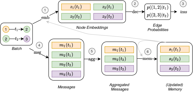
Modelling approach: maintain a memory state for each node, updated upon each interaction. Compute node embeddings on demand for any time \(t\), using only events with timestamp \(\le t\), never later ones.
Examples:
- Reddit posts (user posts to subreddit at timestamp)
- Wikipedia edits (user edits page at timestamp)
- E-commerce interactions (user clicks product at time)
Advantage over snapshots: exact timing information preserved; computation triggered by events (sparse updates).
Key Challenges
1. Evolving Structure
New edges and nodes arrive continuously. The model must incorporate new information without full retraining:
- Transductive: all nodes known at training time
- Inductive: new nodes appear at test time (requires generalising to unseen entities)
2. Temporal Dependencies
Events at time \(t\) may depend on events at \(t - k\) (historical context). Capturing long-range temporal dependencies while maintaining efficient updates is the core challenge.
4. Causality
Every prediction about time \(t\) must be computed from events strictly in the past. Shuffling an event stream before splitting into train and test, as one would for i.i.d. data, leaks future edges into the past and inflates results. Dynamic-graph splits are always chronological.
3. Forgetting and Recency
Not all past events are equally relevant. A social interaction from 3 years ago matters less than one from last week. Models must balance memory capacity with relevance weighting.
Visualising DTDG vs CTDG
DTDG vs CTDG: Practical Trade-offs
| Property | DTDG (Snapshots) | CTDG (Event Stream) |
|---|---|---|
| Temporal resolution | Coarse (snapshot intervals) | Fine (exact timestamps) |
| Modelling complexity | GNN + sequence model | Event-driven memory |
| Computation | Per snapshot (batched) | Per event (online) |
| Handles new nodes | Retrain or fine-tune | Naturally inductive |
| Memory of history | Implicit in sequence model | Explicit memory module |
| Use cases | Regular-interval data | Irregular event data |
Standard Benchmarks
CTDG benchmarks:
- Wikipedia: 9227 nodes, 157474 interaction events
- Reddit: 10984 nodes, 672447 interaction events
- MOOC: student-course interactions with timestamps
- LastFM: user-song interactions (music streaming)
DTDG benchmarks:
- Bitcoin-OTC / Bitcoin-Alpha: trust ratings over time
- DBLP co-authorship: yearly snapshots
- Yelp reviews: monthly snapshots
Summary
| Concept | Definition |
|---|---|
| Static graph | Fixed \((V, E, X)\), standard GNN setting |
| Snapshot graph | Series \(G_1, \dots, G_T\) of static graphs |
| Event stream | Ordered sequence of timestamped interactions |
| Inductive | Generalises to nodes not seen during training |
| Memory module | Fixed-size state capturing interaction history |
Dynamic graph learning adds the temporal dimension to all GNN tasks: link prediction becomes “will \(u\) and \(v\) interact after time \(t\)?”, node classification becomes “what is \(v\)’s state at time \(t\)?”, and graph-level tasks must account for structural evolution. Whatever the task, the model may only look at events with timestamp \(\le t\). TGN is the most widely used CTDG framework and the usual first baseline.
References
- Kazemi, S. M., Goel, R., Jain, K., Kobyzev, I., Sethi, A., Forsyth, P., & Poupart, P. (2020). Representation Learning for Dynamic Graphs: A Survey. JMLR 2020 (comprehensive survey of DTDG and CTDG methods, taxonomy of tasks and models).
- Rossi, E., Chamberlain, B., Frasca, F., Eynard, D., Monti, F., & Bronstein, M. (2020). Temporal Graph Networks for Deep Learning on Dynamic Graphs. ICML GRL+ Workshop 2020 (TGN framework introducing the memory module abstraction).
- Xu, D., Ruan, C., Körpeoglu, E., Kumar, S., & Achan, K. (2020). Inductive Representation Learning on Temporal Graphs. ICLR 2020 (TGAT: temporal graph attention for CTDG without memory modules).