Spatio-Temporal GNNs: Learning on Graphs Through Time

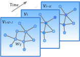
The Spatio-Temporal Setting

Intuition First: Imagine a city-wide network of traffic sensors. At any moment, sensor A reports 30 mph while sensor B (one mile downstream) still reports 60 mph — but in 5 minutes, B will slow down too. A purely temporal model sees each sensor in isolation and misses this propagation. A purely spatial model has no sense of time. ST-GNNs handle both at once: they let each sensor “talk” to its road-network neighbours at every timestep.

Given:

• Fixed graph G = (V, E) — the spatial structure (road network, weather stations)
• Time series at each node: X_t ∈ ℝ^{N × d} for t = 1, …, T
• Goal: predict X_{T+1}, …, X_{T+H} from X_{T-τ+1}, …, X_T

The key insight: sensors at nearby nodes are correlated. A traffic jam upstream affects downstream sensors. A temperature reading in Paris is informative for predicting Frankfurt. The graph structure encodes which nodes influence each other.

Two Architectures

DCRNN (Diffusion Convolutional Recurrent Neural Network)

DCRNN replaces the linear transformation in a GRU with a diffusion convolution — a GNN layer that captures directional information flow:

Standard GRU update:

DCRNN (replace linear with graph conv):

Specifically, DCRNN uses bidirectional random walk diffusion to capture both forward and backward traffic flow directions:

For traffic: forward diffusion follows traffic direction; backward diffusion captures reverse influence.

Encoder-decoder: DCRNN uses an encoder (GRU on past T steps) and a decoder (GRU for future H steps), with scheduled sampling to avoid exposure bias.

STGCN (Spatio-Temporal Graph Convolutional Network)

STGCN alternates spatial (graph convolution) and temporal (1D convolution) blocks:

Input: (N × T × d)
       ↓
Temporal conv (1D across time axis)
       ↓
Spatial conv (GCN across node axis)
       ↓
Temporal conv
       ↓
... repeat
       ↓
Output: (N × H × d)

Each temporal block uses a gated 1D convolution (GLU: gated linear unit) across the time dimension. Each spatial block uses ChebNet or standard GCN across the node dimension.

Advantage over DCRNN: all-convolutional — no recurrence → parallelisable across time steps → much faster training.

Worked Example: One STGCN Step

Setup: 3 sensors (A, B, C) on a road, each with 1 feature (speed in mph). Current readings: A=60, B=30 (jam), C=55. Adjacency A=[0,1,0; 1,0,1; 0,1,0], symmetric.

Temporal gated conv (GLU) — kernel size 3, 1 input channel, 1 output channel: Suppose at times t-2,t-1,t sensor B reads [40, 35, 30]. With kernel weights θ₁=[0.2,0.5,0.3] and θ₂=[0.1,0.3,0.6]:

• Gate input g = 0.2×40 + 0.5×35 + 0.3×30 = 8+17.5+9 = 34.5
• Gating mask σ(0.1×40+0.3×35+0.6×30) = σ(4+10.5+18) = σ(32.5) ≈ 1.0
• Temporal output for B ≈ 34.5 × 1.0 = 34.5

Spatial GCN step (normalised): degree D = diag(1,2,1), Â = D^{-1/2} A D^{-1/2}

• Updated B = mean of A’s and C’s temporal outputs: (60+55)/2 = 57.5 (pulled toward neighbours)
• Interpretation: B’s representation is now influenced by its free-flowing neighbours — the model learns that this discrepancy predicts an upcoming jam spreading to A and C.

Graph Construction for ST-GNNs

The spatial graph is typically constructed from domain knowledge:

Traffic: node = sensor station, edge = road segment (weighted by distance or travel time)

Weather: node = weather station, edge = geographic proximity (threshold by km distance)

Energy: node = power generator/consumer, edge = transmission line

Some methods learn the graph adaptively:

• MTGNN: learns the graph topology jointly with the ST-GNN
• GWaveNet: adaptive adjacency matrix learned from data

Benchmarks

• METR-LA: 207 traffic sensors in Los Angeles, 4 months, 5-minute intervals
• PEMS-BAY: 325 sensors in Bay Area, 6 months
• Solar-Energy: 137 solar plants, 6 months of production data
• Electricity: 321 electricity consumption time series

Standard task: 15/30/60-minute horizon prediction. Metrics: MAE, MAPE, RMSE.

Recent Advances

GWaveNet (Wu et al., 2019): adds an adaptive adjacency matrix (no predefined graph), trained jointly with the rest. This allows the model to capture non-geographic correlations (sensors far apart but behaviourally correlated).

AGCRN (Bai et al., 2020): fully adaptive — learns node-specific patterns and graph structure simultaneously.

GMAN (Zheng et al., 2020): attention-based approach. Replaces GCN with spatial attention and uses temporal attention across time steps.

Summary

Spatio-temporal GNNs are the dominant framework for sensor network prediction — wherever measurements at graph nodes evolve over time and spatial correlations matter. The field is rapidly incorporating Transformer-style attention to replace both spatial and temporal convolutions.

References

• Li, Y., Yu, R., Shahabi, C., & Liu, Y. (2018). Diffusion Convolutional Recurrent Neural Network: Data-Driven Traffic Forecasting. ICLR 2018 (DCRNN: bidirectional diffusion GCN with GRU encoder-decoder for traffic prediction).
• Yu, B., Yin, H., & Zhu, Z. (2018). Spatio-Temporal Graph Convolutional Networks: A Deep Learning Framework for Traffic Forecasting. IJCAI 2018 (STGCN: gated 1D temporal convolution + Chebyshev spatial convolution, fully parallelisable).
• Wu, Z., Pan, S., Long, G., Jiang, J., Chang, X., & Zhang, C. (2020). Connecting the Dots: Multivariate Time Series Forecasting with Graph Neural Networks. KDD 2020 (GWaveNet: adaptive adjacency matrix + dilated causal convolution for long-range temporal patterns).