
GNNs for Recommender Systems
Published:
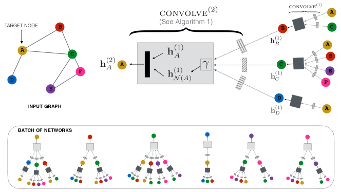
Recommendation as a Graph Problem
Intuition First: Matrix factorisation is like learning that “Alice likes comedies” and “this film is a comedy” and multiplying those two vectors. It captures direct user–item similarity but cannot represent the chain: “Alice liked this film, Bob also liked it, Bob also liked that other film, so Alice might like that other film too.” GNNs capture this multi-hop chain by propagating information along the bipartite graph, 2-hop neighbours of Alice (items liked by users who liked Alice’s items) are exactly the collaborative filtering signal that matrix factorisation misses.
Traditional collaborative filtering: learn a user embedding \(e_u\) and an item embedding \(e_i\), then predict the score as \(\hat{y}_{ui} = e_u^{\top} e_i\). This captures pairwise similarity but not higher-order structure.
GNN approach: build a bipartite graph in which user \(u\) is joined to item \(i\) whenever \(u\) interacted with \(i\). Run a GNN to produce embeddings that capture multi-hop neighbourhood structure:
- 1-hop: items \(u\) has interacted with (or users who interacted with \(i\))
- 2-hop: items interacted with by users who also interacted with \(u\)’s items, the collaborative filtering signal
- 3-hop: transitive similarities
The Bipartite User-Item Graph
Let \(U\) be the users and \(I\) the items, with \(V = U \sqcup I\):
Because the graph is bipartite, message passing alternates sides, users only ever hear from items, and items only from users:
After \(K\) layers, \(h_u^{(K)}\) encodes the \(K\)-hop neighbourhood. Note the parity: odd \(k\) mixes in items, even \(k\) mixes in other users, so it takes at least two layers before any collaborative signal reaches \(u\) at all.
LightGCN (He et al., 2020)
LightGCN makes a key simplification: remove the weight matrices and the non-linearities. Each layer is nothing but symmetrically normalised averaging over the bipartite graph:
The final embedding is a weighted combination of every layer, which is how the model retains the 0-hop signal instead of over-smoothing it away:
Why remove the transformations? Because on these benchmarks there is nothing for them to transform. The paper’s ablation removes \(W_k\) and \(\sigma(\cdot)\) one at a time and finds that each removal helps, with the combined removal helping most: the collaborative signal lives in the propagation, and extra learnable matrices mainly add capacity to overfit.
PinSage (Ying et al., 2018)
Pinterest’s GNN for image recommendation, and one of the first published industrial deployments of a GNN.
Scale: the paper reports a bipartite pin–board graph of 3 billion nodes and roughly 18 billion edges.
Key innovations:
- GraphSAGE-style sampling: for each node, sample a fixed-size neighbourhood rather than the full one, this is what makes the computation tractable, since a full-neighbourhood pass over a graph this size is hopeless
- Random-walk importance sampling: choose neighbours by how often they are visited in short random walks from the target node, not uniformly, and weight their messages by that visit count
- Curriculum training: feed progressively harder negative examples as training proceeds
NGCF and Variants
NGCF (Wang et al., 2019): adds an explicit feature interaction to the message:
The Hadamard product \(h_i \odot h_u\) is meant to capture user-item feature interaction. LightGCN’s ablation found that on the standard collaborative-filtering benchmarks this term costs more in overfitting than it returns in expressiveness, though the argument is specific to the ID-embedding-only setting, and richer side features change the calculus.
Session-Based Recommendation
Standard CF assumes all past interactions are known for each user. Session-based recommendation has no long-term user history, only the current session (sequence of clicks).
SR-GNN (Wu et al., 2019): model a session as a directed graph (clicks are edges from previous item to next item). Run GCN on session graph, then use attention to extract user intent from node embeddings. This captures transition patterns between items within a session.
Knowledge Graph-Enhanced Recommendation
KGNN-LS / KGCN: enrich the item side with a knowledge graph (item → category, brand, attributes). GNN propagates over both the user-item graph and the item knowledge graph simultaneously.
Benefit: cold-start items with no interactions can leverage KG features (genre, director for movies) to receive recommendations from users with similar taste in KG-related items.
Summary
| Model | Key idea | Hops used |
|---|---|---|
| Matrix factorisation | Pairwise similarity only | 0 (direct inner product) |
| NGCF | GCN + explicit feature interaction | \(K\) hops, with \(W_1, W_2\) per layer |
| LightGCN | Normalised propagation, no \(W\) or \(\sigma\) | \(K\) hops, layer-combined |
| PinSage | GraphSAGE + random-walk importance sampling | Sampled 2-hop neighbourhoods |
| SR-GNN | Session graph + gated GNN | Within-session transitions |
The mechanism that unifies these is the one worth remembering: on a bipartite interaction graph, a \(K\)-layer GNN gives every user an embedding that already contains the items liked by users like them. That is collaborative filtering expressed as message passing, and it is why PinSage could be deployed at Pinterest’s graph scale while a dense user-item matrix could not.
References
- Ying, R., He, R., Chen, K., Eksombatchai, P., Hamilton, W. L., & Leskovec, J. (2018). Graph Convolutional Neural Networks for Web-Scale Recommender Systems. KDD 2018 (PinSage: GraphSAGE-based GNN for Pinterest’s 3-billion-node pin-board graph at production scale).
- He, X., Deng, K., Wang, X., Li, Y., Zhang, Y., & Wang, M. (2020). LightGCN: Simplifying and Powering Graph Convolution Network for Recommendation. SIGIR 2020 (LightGCN: ablation study showing that removing feature transformation and activation from GCN improves collaborative filtering).
- Wu, S., Tang, Y., Zhu, Y., Wang, L., Xie, X., & Tan, T. (2019). Session-Based Recommendation with Graph Neural Networks. AAAI 2019 (SR-GNN: models session sequences as directed graphs for next-item prediction with GNN).