
Global Pooling in GNNs: Mean, Sum, and Max
Published:
Intuition First: Summarising a Set of Vectors
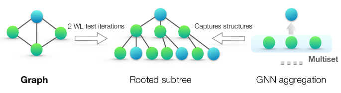
After message passing you have a bag of node embeddings, an unordered set of vectors. You need to compress this whole set into a single fixed-size vector. Think of it like summarising a group of people: you could report the average height (mean), the total weight (sum), or the tallest person (max). Each statistic captures different information, and each is lossy in a different way. The same is true for graph readout.
The Readout Problem
A \(K\)-layer GNN produces a set of node embeddings \(\{h_v^{(K)} : v \in V\}\), equivalently the layer matrix \(H^{(K)} \in \mathbb{R}^{N \times d}\) with one row per node. For node-level tasks (node classification, link prediction), these are used directly. For graph-level tasks (graph classification, graph regression), they must be compressed into a single vector \(h_G\).
This compression is the readout or global pooling step. It must be:
- Permutation-invariant: the same graph regardless of node ordering
- Differentiable: end-to-end training
- Expressive: different graphs should map to different embeddings
Mean Pooling
Properties:
- Permutation-invariant: yes
- Normalised by graph size: yes (divides by \(\lvert V \rvert\))
- Sensitive to graph size: no, a graph with 10 identical nodes and one with 100 identical nodes give the same embedding
- Captures average node behaviour
When to use: tasks where the typical node matters, e.g., average atom property in a molecule, average sentiment in a document graph.
Failure case: cannot distinguish a graph with one active node from a graph with 100 identical active nodes, mean pooling normalises out the count.
Sum Pooling
Properties:
- Permutation-invariant: yes
- Sensitive to graph size: yes (more nodes → larger magnitude)
- Injective over multisets: yes, when composed with a learnable node-wise transform and the feature space is countable
- Captures total contribution of all nodes
When to use: tasks where the total matters, e.g., total charge of a molecule, total influence in a social network.
Expressive power: Xu et al. (GIN, 2019) show that a readout of the form \(h_G = \sum_{v} \phi(h_v^{(K)})\) with a learnable \(\phi\) can represent any function of the multiset of node embeddings, provided the embeddings come from a countable set. Neither mean nor max has that property: mean discards multiplicities, max discards everything but the per-dimension extremes.
Failure case: the magnitude of \(h_G\) scales with \(\lvert V \rvert\), so a downstream MLP sees inputs whose scale varies across the dataset. Nodes with near-zero embeddings also contribute nothing, so sum cannot separate a graph with 10 such nodes from one with 100.
Max Pooling
Properties:
- Permutation-invariant: yes
- Captures the most prominent feature value in each dimension
- Insensitive to count of nodes with non-maximal features
When to use: tasks where the extreme matters, e.g., is there any toxic functional group? Does any node have property X?
Failure case: cannot distinguish \(\{1, 2\}\) from \(\{2\}\), max pooling drops information about non-maximal elements.
Expressivity Ranking
Composed with a learnable node-wise transform, sum readout is the most expressive of the three: it is the only one of them that can represent an arbitrary function of the multiset of node embeddings drawn from a countable universe. This is what allows GIN to reach the 1-WL bound at graph level, and 1-WL is an upper bound on what any message-passing GNN can distinguish.
Compared as bare statistics, though, mean and max are not simply “weaker than sum”: they are incomparable to each other, and each separates some multisets that sum does not.
| Multiset pair | Mean | Max | Sum |
|---|---|---|---|
| \(\{1\}\) vs \(\{1,1,1\}\) | same | same | different |
| \(\{1,3\}\) vs \(\{2,2\}\) | same | different | same |
| \(\{1,2\}\) vs \(\{2\}\) | different | same | different |
The practical reading: sum is the safe default because a learned \(\phi\) can always recover mean-like or max-like behaviour from it, but only if the network is given the capacity to do so.
Combinations and Hierarchical Pooling
In practice, combining multiple pooling types often works best:
h_G = concat( mean_pool(H), sum_pool(H), max_pool(H) )
This captures average behaviour (mean), count sensitivity (sum), and extreme values (max) simultaneously.
For graphs where structure at different scales matters (molecules with atoms and functional groups, social networks with individuals and communities), hierarchical pooling, covered in DiffPool and TopK-Pool posts, is more appropriate than flat global pooling.
Summary
| Pooling | Formula | Sensitive to Size | Information Captured | Best For |
|---|---|---|---|---|
| Mean | \(\frac{1}{\lvert V\rvert}\sum_v h_v\) | No | Average node behaviour | Distribution of properties |
| Sum | \(\sum_v h_v\) | Yes | Total + count | Additive properties |
| Max | \(\max_v h_v\) (elementwise) | No | Extreme values | Existence queries |
| Concat(all) | \([\,\text{mean};\text{sum};\text{max}\,]\) | Partial | Combined | General tasks |
The choice of readout is as important as the choice of message passing architecture: on graph-level tasks where the count of a substructure is what the label depends on, swapping mean for sum is the difference between a model that can express the target function and one that provably cannot, no amount of extra message-passing depth compensates for a readout that has already thrown the information away.
References
- Xu, K., Hu, W., Leskovec, J., & Jegelka, S. (2019). How Powerful are Graph Neural Networks?. ICLR 2019 (sum aggregation with a learnable transform is injective over multisets; mean and max are not).
- Zaheer, M., Kottur, S., Ravanbakhsh, S., Poczos, B., Salakhutdinov, R., & Smola, A. J. (2017). Deep Sets. NeurIPS 2017 (theory of permutation-invariant functions over sets).