
DiffPool: Learning Hierarchical Graph Pooling
Published:
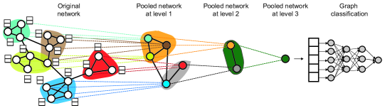
Intuition First: Hierarchical Pooling as a Convolutional Pyramid
In image CNNs, max-pooling after each conv layer progressively coarsens the spatial grid: \(32 \times 32 \to 16 \times 16 \to 8 \times 8 \to 1 \times 1\). This captures multi-scale features, edges at fine scale, shapes at coarser scale, objects at the coarsest. DiffPool brings this pyramid idea to graphs: \(\text{nodes} \to \text{clusters} \to \text{super-clusters} \to \text{graph}\). The key challenge is that unlike pixels, graph nodes have no fixed spatial ordering, so the pooling must be learned and permutation-invariant.
The Limitation of Flat Global Pooling
Global mean/sum/max pooling jumps directly from \(N\) node embeddings to a single graph embedding. For graphs with hierarchical structure, like molecules (atoms → functional groups → whole molecule) or social networks (people → communities → factions), this skips all intermediate scales.
CNNs solve this with hierarchical pooling (max-pool after each conv layer). DiffPool brings the same idea to graphs, with the key challenge: graph pooling must be permutation-invariant and must handle variable numbers of nodes.
The DiffPool Architecture
DiffPool processes each pooling level \(l\) with two GNNs, both run on the same inputs, the level’s adjacency \(A^{(l)} \in \mathbb{R}^{N_l \times N_l}\) and its node feature matrix \(X^{(l)} \in \mathbb{R}^{N_l \times d}\) (at the first level, \(X^{(0)} = X\) and \(A^{(0)} = A\)).
1. Embedding GNN, computes node embeddings:
2. Pooling GNN, computes cluster assignments:
\(S^{(l)}\) is the soft assignment matrix: \(S^{(l)}_{ij}\) is the probability that node \(i\) at level \(l\) belongs to cluster \(j\) at level \(l+1\). The softmax is applied row-wise, so every row sums to one, each node distributes a unit of “mass” across the \(k_l\) clusters. Note that the two GNNs share an architecture but not weights: one is trained to produce features, the other to produce a clustering.
Coarsening: the assignment matrix is then used twice, once to pool features, once to pool the graph:
\(X^{(l+1)}\) is the input feature matrix of the next level: each cluster’s embedding is the assignment-weighted sum of its member nodes’ embeddings. The new adjacency \(A^{(l+1)}\) is the cluster-to-cluster connectivity, entry \((a,b)\) accumulates the edge weight between clusters \(a\) and \(b\) over all pairs of constituent nodes. Because \(S^{(l)}\) is dense, \(A^{(l+1)}\) is a dense weighted adjacency even when \(A^{(l)}\) was sparse.
Why Soft Assignment?
Hard assignment (each node assigned to exactly one cluster) would require an \(\arg\max\), not differentiable. Soft assignment (each node fractionally assigned to all clusters) allows end-to-end gradient flow.
The assignment \(S^{(l)}\) is learned jointly with the rest of the network. The model discovers which nodes should be clustered together, without any external supervision on the clustering.
Auxiliary Loss Terms
Nothing in the architecture so far forces \(S^{(l)}\) to be a sensible clustering, a degenerate assignment that spreads every node uniformly over all clusters is perfectly differentiable and perfectly useless. DiffPool therefore adds two auxiliary losses, minimised alongside the task loss at every pooling layer.
Auxiliary link prediction loss: encourages nodes connected by an edge to be assigned to the same cluster:
\(\bigl(S^{(l)}S^{(l)\top}\bigr)_{ij}\) is the probability that nodes \(i\) and \(j\) land in the same cluster. Pushing that matrix towards \(A^{(l)}\) makes the clustering agree with the observed edges, so clusters correspond to densely connected regions rather than arbitrary groups of nodes. The name is a little misleading: no link prediction task is being solved, it is a regulariser that reads the adjacency as a target.
Entropy loss: encourages each node’s assignment to be concentrated rather than uniformly spread:
where \(S^{(l)}_i\) is row \(i\) of the assignment matrix. Minimising \(L_E\) drives each row towards a one-hot vector, so the soft assignment approaches a hard clustering as training progresses, sharper clusters, and a coarsened adjacency that is less blurred.
Concrete Worked Example: One DiffPool Step
Suppose we have 4 nodes and want to pool to 2 clusters. After the embedding GNN, the node embeddings are \(Z \in \mathbb{R}^{4 \times 3}\):
Z = [[1, 0, 1],   # node 0
     [1, 0, 0],   # node 1, similar to node 0
     [0, 1, 1],   # node 2
     [0, 1, 0]]   # node 3, similar to node 2
The pooling GNN outputs raw logits; the row-wise softmax turns them into the assignment \(S \in \mathbb{R}^{4 \times 2}\):
S = [[0.9, 0.1],   # node 0 → mostly cluster A
     [0.8, 0.2],   # node 1 → mostly cluster A
     [0.1, 0.9],   # node 2 → mostly cluster B
     [0.2, 0.8]]   # node 3 → mostly cluster B
New cluster features: \(X' = S^{\top} Z \in \mathbb{R}^{2 \times 3}\). Each row of \(X'\) is the column of \(S\) for that cluster, used as weights over the rows of \(Z\):
X'[A] = 0.9×[1,0,1] + 0.8×[1,0,0] + 0.1×[0,1,1] + 0.2×[0,1,0]
      = [1.7, 0.3, 1.0]   (cluster A = nodes 0+1)
X'[B] = 0.1×[1,0,1] + 0.2×[1,0,0] + 0.9×[0,1,1] + 0.8×[0,1,0]
      = [0.3, 1.7, 1.0]   (cluster B = nodes 2+3)
The soft assignment correctly merged structurally similar nodes (0,1) into cluster A and (2,3) into cluster B, learned purely from features and graph structure. Note that the two clusters agree exactly in the third coordinate: that dimension was uninformative about the split, and the pooling reflects that rather than manufacturing a difference.
Computational Cost
DiffPool runs two GNNs at each level. For a graph with \(N\) nodes coarsened to \(k\) clusters:
- Assignment: \(S \in \mathbb{R}^{N \times k}\) is dense, \(O(Nk)\) entries, and every node has a nonzero weight on every cluster.
- Coarsening the adjacency: \(S^{\top} A S\) costs \(O(N^2 k)\) with a dense \(A\), and produces a dense \(k \times k\) result.
- Memory: \(O(N^2)\), the dominant term is the dense adjacency \(A^{(l)}\) itself, which DiffPool requires because \(A^{(l+1)}\) is dense from the second level onward regardless of how sparse the input graph was.
This \(O(N^2)\) memory cost is the defining practical constraint. It is not an implementation detail that a better sparse kernel could remove: the soft assignment genuinely connects every cluster to every node, so the coarsened graph is genuinely dense. Batching compounds it, graphs in a batch must be padded to a common \(N_{\max}\). DiffPool is therefore practical for graphs with hundreds of nodes (molecules, proteins) but not for social networks or knowledge graphs with millions.
When DiffPool Helps
DiffPool outperforms flat pooling when:
- The task requires multi-scale understanding: molecular property prediction benefits from atom-level and functional-group-level representations simultaneously
- Graphs have natural hierarchical structure: trees, clustered communities, hierarchical molecules
- The graph is small enough: typically a few hundred to a thousand nodes
It remains a standard reference point on the TUDataset graph classification benchmarks the original paper used, ENZYMES, D&D, PROTEINS, COLLAB and REDDIT-MULTI-12K.
Limitations
- Quadratic memory: no scaling to large graphs
- Fixed number of clusters: \(k_l\) must be chosen per level before training, and since the same \(k_l\) applies to every graph in the dataset it is usually set from a percentage of the largest graph
- No guarantee of meaningful clusters: the auxiliary losses help but do not force semantically meaningful groupings
- Sensitive to the number of pooling levels: too many levels → over-compression; too few → flat pooling
Summary
| Component | Role |
|---|---|
| \(\mathrm{GNN}_{l,\text{embed}}\) | Compute node representations at this scale |
| \(\mathrm{GNN}_{l,\text{pool}}\) | Learn soft cluster assignments \(S^{(l)}\) |
| \(X^{(l+1)} = S^{(l)\top} Z^{(l)}\) | Aggregate node embeddings into cluster embeddings |
| \(A^{(l+1)} = S^{(l)\top} A^{(l)} S^{(l)}\) | Coarsen adjacency to cluster graph |
| \(L_{\mathrm{LP}} + L_{E}\) | Encourage connectivity-aligned, sharp clusters |
DiffPool introduced the idea of learned hierarchical pooling for graphs, differentiable, end-to-end, and structure-aware. Its quadratic complexity limits scale, but for small-graph tasks (molecules, proteins), it remains a reference architecture.
References
- Ying, R., You, J., Morris, C., Ren, X., Hamilton, W. L., & Leskovec, J. (2018). Hierarchical Graph Representation Learning with Differentiable Pooling. NeurIPS 2018.
- Simonovsky, M., & Komodakis, N. (2017). Dynamic Edge-Conditioned Filters in Convolutional Neural Networks on Graphs. CVPR 2017.