Why Some Graphs Fool GNNs: The Structural Indistinguishability Problem

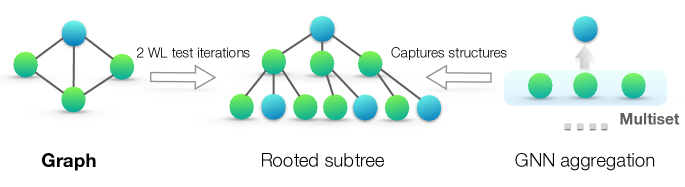
Intuition First

The 1-WL test works by giving every node a “colour” based on its neighbourhood multiset, then iteratively refining colours. Two nodes get the same final colour if and only if their entire computational trees — the tree of all neighbours’ neighbours’ neighbours… — look identical.

The catch: a tree cannot see cycles. A node in a triangle and a node with the same three neighbours but no triangle between them have identical computational trees at depth 1. And since GNNs are equivalent to 1-WL, GNNs are cycle-blind.

The Expressivity Ceiling

The Weisfeiler-Lehman (1-WL) test is the exact expressivity ceiling for message-passing GNNs. Two graphs that 1-WL cannot distinguish cannot be distinguished by any MPNN — including GCN, GAT, GIN.

This is not a theorem about bad architectures. Even the most expressive MPNN (GIN) is bounded by 1-WL. The question becomes: what does 1-WL fail to distinguish?

Case 1: Regular Graphs

A k-regular graph is a graph where every node has degree k. When all nodes have the same degree, they start with identical initial colours in 1-WL. After one iteration, every node sees k neighbours, all with the same colour → same colour update. After any number of iterations: all nodes still have the same colour.

Consequence: Any two k-regular graphs with the same number of nodes and edges get the same 1-WL histogram — and thus the same graph-level embedding in any MPNN.

Graph A: Triangle (3 nodes, 3 edges, 2-regular)
Graph B: Three disjoint edges (6 nodes, 3 edges, 1-regular)
→ Different (1-WL can distinguish these: different degree)

Graph C: Petersen graph (10 nodes, 15 edges, 3-regular)
Graph D: Different 3-regular graph on 10 nodes, 15 edges
→ SAME 1-WL signature — any MPNN predicts identically for graph-level tasks

For molecular graphs (where degree encodes atom valence), this means two chemically distinct molecules with the same degree sequence can be indistinguishable.

Case 2: Cycle Counting Blindness

1-WL cannot count cycles. Specifically:

A 4-cycle and two disconnected edges look identical to 1-WL if node features are uniform:

4-cycle: A-B-C-D-A  (all degree-2)
Two edges: A-B, C-D  (all degree-1)

These ARE distinguishable (different degrees). But:

6-cycle: A-B-C-D-E-F-A  (2-regular)
Two 3-cycles: {A-B-C-A} ∪ {D-E-F-D}  (2-regular)

Both are 2-regular with 6 nodes and 6 edges. 1-WL assigns identical histograms. No MPNN can distinguish them — but they are structurally very different (one is connected, one is not… wait, both are).

Actually for the connected case: a 6-cycle has no triangles; two 3-cycles has two triangles. An MPNN cannot detect whether nodes are in triangles unless it uses structural encodings or higher-order methods.

Case 3: The CSL Graph Family

The Circular Skip Link (CSL) graphs are a family of 4-regular graphs on 41 nodes. They all look identical to 1-WL — every node has degree 4, the neighbourhood multisets match at every depth.

Yet the graphs are non-isomorphic (they have different skip patterns). Tasks that require distinguishing them (e.g., graph classification) will be solved at chance level by any MPNN.

CSL is a standard benchmark for testing beyond-1-WL expressiveness.

Concrete Failure: Molecule Classification

Suppose two molecules both have 6 carbon atoms, each with exactly 2 bonds (degree-2). One is benzene (a 6-cycle, aromatic), the other is two propene fragments (two 3-cycles). Both have the same 1-WL colour histogram.

A GNN trained to predict aromaticity will assign these the same graph-level embedding — and therefore the same prediction — even though only benzene is aromatic. This is not a data issue; it is a fundamental architectural limit.

The fix: add ring-membership features (e.g., RWPE captures P³[v,v] > 0 for nodes in triangles) or use subgraph GNNs that explicitly detect cycles.

Why This Matters in Practice

For graph classification (e.g., is this molecule toxic?):

• Two molecules with different structures but same 1-WL signature → same MPNN prediction
• If the toxicity mechanism involves a structural feature 1-WL cannot detect → systematic failure

For node classification in a regular graph:

• All nodes have the same embedding → the GNN cannot distinguish any nodes at all
• If labels differ between nodes, accuracy collapses to the majority class

For link prediction in a regular graph:

• All node pairs have the same score → random link prediction

What Structural Features Are Invisible?

1-WL cannot detect:

• Cycle lengths (is a node in a 4-cycle vs 6-cycle?)
• Triangle counts (how many triangles contain node v?)
• Clique membership (is v in a clique?)
• Global structural roles (is v a bridge node? is it on the periphery?)
• Non-local symmetries (two nodes with identical local neighbourhoods but different global positions)

Solutions

Structural positional encodings (random walk PE, Laplacian PE) inject node-level structural identity that breaks the symmetry 1-WL cannot break — at the cost of sign/basis ambiguity issues.

Subgraph GNNs run a GNN on each induced subgraph and pool results — provably more expressive than 1-WL but O(N²) or O(N³) in complexity.

Summary

Knowing which graphs fool GNNs is not just academic — it directly predicts where standard GNNs will fail on real tasks, and which architectural upgrades are needed.

References

• Xu, K., Hu, W., Leskovec, J., & Jegelka, S. (2019). How Powerful are Graph Neural Networks?. ICLR 2019.
• Murphy, R. L., Srinivasan, B., Rao, V., & Ribeiro, B. (2019). Relational Pooling for Graph Representations. ICML 2019 (on k-WL and beyond-1-WL methods).
• Maron, H., Ben-Hamu, H., Serviansky, H., & Lipman, Y. (2019). Provably Powerful Graph Networks. NeurIPS 2019.