
SGC: Simple Graph Convolution
Published:
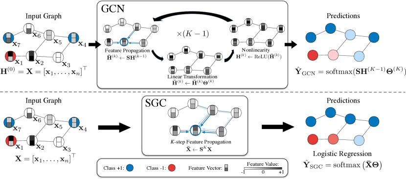
The GCN Formula Revisited
GCN with K layers applies:
Where S̃ = D̃^{-1/2} Ã D̃^{-1/2} is the normalised adjacency with self-loops, and σ is ReLU.
Each layer: (1) aggregate from neighbours (S̃ H^{(k)}), (2) apply a linear transformation W^{(k)}, (3) apply nonlinearity σ.
The nonlinearity σ couples the graph propagation and the linear transformation — you cannot separate or pre-compute them.
The SGC Simplification
SGC (Simple Graph Convolution) makes two changes:
- Remove all intermediate nonlinearities
- Collapse all weight matrices into one
Where S̃ᴷ = S̃ · S̃ · … · S̃ (K times) is the K-th power of the normalised adjacency.
The entire model is now:
- Pre-compute S̃ᴷ X (K steps of feature propagation — this is a fixed linear operation)
- Apply a single linear classifier W to the smoothed features
- Softmax for probabilities
Concrete example showing the collapse. For a 3-layer GCN with weight matrices W₀, W₁, W₂ and ReLU activations:
GCN (3 layers):
  H¹ = ReLU( S̃ · X  · W₀ )     ← cannot pre-compute (W₀ is inside ReLU)
  H² = ReLU( S̃ · H¹ · W₁ )     ← depends on H¹
  H³ = ReLU( S̃ · H² · W₂ )     ← depends on H²

SGC (K=3): remove all intermediate nonlinearities, collapse all W:
  X̃ = S̃³ · X                    ← pre-compute ONCE (no parameters!)
  Ŷ = softmax( X̃ · W )          ← single linear layer trained on cached X̃
| Pre-computation time: O(3· | E | ·d) run once before training. Per-epoch cost: just O(N·d·C) — logistic regression speed. |
Pre-Computation: The Key Efficiency Gain
Because S̃ᴷ X involves no learned parameters, it can be computed once before training and cached. Training then reduces to logistic regression on the pre-computed features S̃ᴷ X.
Computational cost comparison (training, N nodes, K=2):
| Model | Forward pass cost | ||
|---|---|---|---|
| GCN (2 layers) | O( | E | · d₁ + N · d₁ · d₂) |
| SGC (K=2) | **O( | E | · d)** pre-compute, then O(N · d · C) per epoch |
For Cora (2,708 nodes, 10,556 edges): SGC is 11× faster than GCN with similar accuracy.
Theoretical Interpretation
S̃ᴷ X is a K-step random walk smoothing of node features. Each application of S̃ moves each node’s feature vector toward the weighted average of its neighbours. After K steps, each node’s feature is a weighted average over its K-hop neighbourhood.
SGC then applies a linear classifier on this smoothed representation — exactly analogous to a linear classifier on bag-of-words features, where the “bag” is the K-hop neighbourhood.
When Nonlinearities Do Matter
SGC’s simplification works on homophilic graphs (Cora, CiteSeer, Pubmed). On these, K-step averaging makes same-class nodes progressively more similar — which is exactly what the linear classifier needs.
SGC fails relative to GCN on:
- Heterophilic graphs: averaging across class boundaries hurts
- Complex structural tasks: tasks where the pattern is in the local structure, not smooth features
- Very deep propagation: without nonlinearities, K-step averaging becomes over-smoothing very quickly
SGC as Logistic Regression
After pre-computing X̃ = S̃ᴷ X, the SGC model is:
This is exactly logistic regression on pre-computed graph-smoothed features. The model has no architecture hyperparameters beyond K. There is no depth, no hidden layers, no dropout decisions.
This makes SGC the perfect ablation baseline: if SGC matches your GNN, the GNN’s complexity is not providing value.
SGC Variants and Successors
- SIGN (2020): use multiple powers of S̃ simultaneously (X, S̃X, S̃²X, …) and concatenate, then apply an MLP. More expressive than SGC while keeping pre-computation.
- APPNP: separate propagation from transformation with personalized PageRank.
- GAMLP: large-scale variant using multiple propagation matrices.
Summary
| Property | GCN | SGC |
|---|---|---|
| Per-layer nonlinearity | Yes (ReLU) | No |
| Weight matrices | K separate W^{(k)} | Single W |
| Propagation pre-computable | No | Yes |
| Training cost | High (full forward pass) | Low (logistic regression) |
| Accuracy (homophilic) | Slightly better | Comparable |
| Accuracy (heterophilic) | Poor | Also poor |
SGC reveals that graph neural networks, at least in the homophilic setting, are largely doing one thing: smoothing features over the graph and then classifying. The sophistication of multi-layer nonlinear GNNs can sometimes be simplified to this without loss — a profound insight about what graph learning actually requires.
References
- Wu, F., Zhang, T., de Souza Jr., A. H., Fifty, C., Yu, T., & Weinberger, K. Q. (2019). Simplifying Graph Convolutional Networks. ICML 2019.
- Kipf, T. N., & Welling, M. (2017). Semi-Supervised Classification with Graph Convolutional Networks. ICLR 2017.