
Oversquashing: When Too Much Information Passes Through Bottlenecks
Published:
Intuition First: The Telephone Game Through a Bottleneck
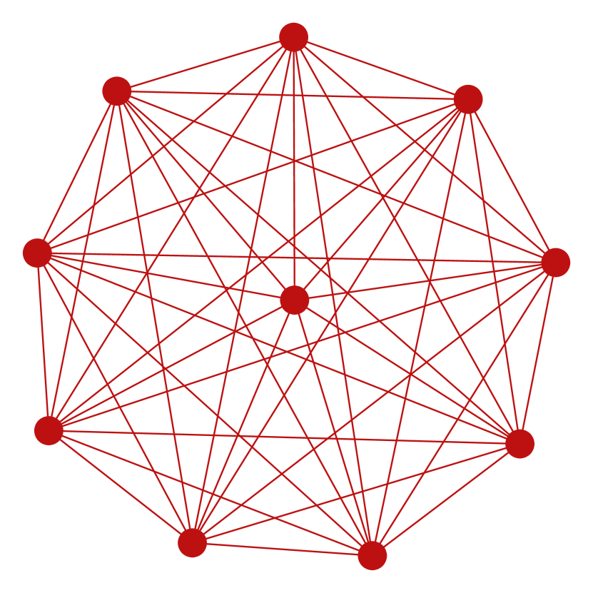
Imagine passing a message through a chain of people, but at one point the chain narrows to a single person who must relay messages from 1,000 people on one side to 1,000 people on the other. That single relay is a bottleneck: the message each person on the far side receives is an extremely compressed, noisy version of the original. Oversquashing is exactly this, distant node information must squeeze through bottleneck edges into a fixed-size embedding, losing fidelity exponentially with distance.
Two Different Problems
Oversmoothing (too many layers → embeddings converge) and oversquashing (long-range info is lost at bottlenecks) are often confused. They are distinct:
| Oversmoothing | Oversquashing | |
|---|---|---|
| Cause | Iterated averaging → feature collapse | Neighbourhood growth + bottlenecks → info compression |
| Affects | Nearby nodes most | Distant nodes most |
| More layers | Makes it worse | Would help (more hops) but also squashes more |
| Root mechanism | Low-pass filtering | Information bottleneck |
| Formal object | Spectrum of \(\hat{A}\): \(\hat{A}^K \to u_1u_1^{\top}\) | Jacobian: \(\lVert \partial h_v^{(K)}/\partial x_u \rVert \to 0\) |
| Graph structure involved | Dense, connected graphs | Narrow bottleneck edges |
The Exponential Growth Problem
In a \(K\)-layer MPNN, node \(v\)’s embedding \(h_v^{(K)}\) depends on every node within \(K\) hops, its receptive field \(\mathcal{N}_K(v)\). On a graph that is locally tree-like with branching factor \(d\), that set grows exponentially:
where \(p\) is the fixed hidden width. The width \(p\) does not grow with \(K\), so the information any single distant node \(u\) can claim shrinks roughly like \(1/d^{K}\). Even if \(u\)’s feature is critical for predicting \(v\)’s label, it is drowned out.
Note the condition: this exponential argument needs the neighbourhood to actually expand. On a path or a cycle, \(\lvert\mathcal{N}_K(v)\rvert\) grows only linearly, and oversquashing there arises from a different mechanism, the decay of the propagation operator over distance, quantified next.
The Jacobian Analysis
Alon & Yahav (2021) identified and named oversquashing; Topping et al. (2022) made it quantitative by bounding the Jacobian
which measures how sensitive \(v\)’s \(K\)-layer embedding is to \(u\)’s input feature \(x_u\). Unrolling \(K\) layers of message passing gives a bound of the form
where \(w\) bounds the norms of the weight matrices, \(c\) bounds the Lipschitz constant of the non-linearity, and \(\hat{A} = \tilde{D}^{-1/2}\tilde{A}\tilde{D}^{-1/2}\) is the same propagation matrix as in the oversmoothing post. The topology enters through the single factor \((\hat{A}^{K})_{vu}\).
Two consequences follow. First, if \(u\) is more than \(K\) hops from \(v\) then \((\hat{A}^{K})_{vu} = 0\) exactly, no amount of training can create sensitivity that the receptive field does not contain. Second, when \(u\) is reachable but only through a bottleneck, \((\hat{A}^{K})_{vu}\) is tiny, so the forward signal and the gradient \(\partial \mathcal{L}/\partial x_u\) are both suppressed: the model cannot learn that \(u\) matters for \(v\).
Where Oversquashing Is Severe
Oversquashing is worst when:
- The path between relevant nodes is long (diameter » number of layers)
- Bottleneck edges connect high-degree subtrees, many nodes compete through a single edge
- The graph has tree-like structure (few cycles, exponential neighbourhood growth)
Real examples where this matters:
- Molecular property prediction: computing HOMO-LUMO gap requires whole-molecule reasoning; bottleneck edges are single bonds connecting large fragments
- Social network influence: influence travels through single bridges between communities
- Traffic forecasting: a road closure (bottleneck) affects distant nodes but the effect is diluted through many competing paths
Concrete Worked Example: Jacobian Decay on a Path
Take the path graph on 6 nodes, 1–2–3–4–5–6, and ask how much node 1 can influence node 6, which is 5 hops away. Suppose each message-passing step multiplies by a weight matrix with \(\lVert W \rVert = 0.9\) and the non-linearity is 1-Lipschitz, so the bound above reads \(0.9^{K}\,(\hat{A}^{K})_{6,1}\).
The degrees on this path are \((1,2,2,2,2,1)\), so with self-loops \(\tilde{d} = (2,3,3,3,3,2)\). Computing the relevant entries of \(\hat{A}^{K}\) directly:
| Pair | Hops | \((\hat{A}^{K})_{vu}\) | Bound \(0.9^{K}(\hat{A}^{K})_{vu}\) |
|---|---|---|---|
| \(1 \to 2\) | 1 | \(1/\sqrt{6} \approx 0.408\) | \(0.9 \times 0.408 \approx 0.367\) |
| \(1 \to 6\) | 5 | \(\approx 0.00617\) | \(0.9^{5} \times 0.00617 \approx 0.00365\) |
Node 6’s embedding is roughly 100× less sensitive to node 1’s feature than node 2’s is, and the gap widens geometrically with distance. If node 1’s feature is the critical signal for a prediction at node 6, it is effectively invisible to the model.
Notice that most of the decay here comes from \((\hat{A}^{K})_{vu}\), not from the weight norms: even with \(\lVert W\rVert = 1\) the ratio would be \(0.408 / 0.00617 \approx 66\). The topology is doing the damage.
Measuring Oversquashing
The sensitivity score \(\lVert \partial h_v^{(K)} / \partial x_u \rVert\) measures how much node \(u\) influences node \(v\) after \(K\) layers. Plotting it for all pairs \((u,v)\) reveals which edges are bottlenecks.
Two topology-only proxies avoid training a model at all:
- Commute time \(\tau(u,v)\), the expected number of steps for a random walk to go from \(u\) to \(v\) and back. High commute time means information struggles to flow between them.
- Effective resistance \(R(u,v)\), the resistance between \(u\) and \(v\) when each edge is a unit resistor. The two are proportional, \(\tau(u,v) = 2\lvert E\rvert\, R(u,v)\), and effective resistance is the quantity that later work (Di Giovanni et al., 2023) ties directly to oversquashing: pairs separated by high effective resistance are exactly the pairs whose Jacobian is provably small.
Solutions: Graph Rewiring
Graph rewiring adds or removes edges to reduce bottlenecks:
- SDRF (Stochastic Discrete Ricci Flow): adds edges around the most negatively curved edges, edges with negative curvature are bottlenecks
- DIGL: adds edges between nodes with high personalized PageRank similarity
- CurvDrop: removes edges with high negative curvature (bottlenecks) and adds long-range connections
Other approaches:
- Global attention (Graph Transformers): bypasses all bottlenecks, every node attends to every node directly
- APPNP: personalized PageRank allows distant information to flow via many paths simultaneously
- Virtual node: add a single virtual node connected to all other nodes, providing a global communication channel
Curvature and Oversquashing
Topping et al. (2022) connected oversquashing to a notion of discrete Ricci curvature. They introduce the balanced Forman curvature \(\mathrm{Ric}(u,v)\) of an edge, a combinatorial quantity built from the degrees \(d_u, d_v\), the number of triangles containing \((u,v)\), and the 4-cycles through it. An edge is negatively curved when its endpoints share few common neighbours and few short cycles: locally, the edge is the only route between two otherwise separate regions.
The link to oversquashing runs through the Jacobian bound above. Their result is a conditional one, not a blanket guarantee: for a graph containing a sufficiently negatively curved edge, they prove an upper bound on \(\lVert \partial h_v^{(K)}/\partial x_u \rVert\) for pairs \(u,v\) on opposite sides of it, and show that a curvature-guided rewiring (SDRF) increases the curvature of the worst edges. That improves the bound; it does not prove that a trained model’s downstream accuracy must improve. What it does establish is the direction of the connection, from graph geometry (curvature) to information flow (oversquashing).
Summary
| Property | Value |
|---|---|
| Root cause | Receptive-field growth and bottleneck topology vs. fixed embedding width |
| Formal measure | \(\lVert \partial h_v^{(K)}/\partial x_u \rVert \le (cw)^{K}(\hat{A}^{K})_{vu}\), decaying geometrically |
| Topological proxies | Effective resistance \(R(u,v)\), commute time \(\tau(u,v)\), negative edge curvature |
| Worst cases | Long paths, tree-like graphs, single bottleneck bridges |
| Effect | Distant relevant information lost; gradient vanishes |
| Solution 1 | Graph rewiring (add/remove edges) |
| Solution 2 | Global attention (Graph Transformers) |
| Solution 3 | Virtual nodes (global communication channel) |
| Relation to oversmoothing | Distinct: affects different nodes, different depth regime |
Oversquashing explains why GNNs fail on long-range reasoning tasks even when depth is not the bottleneck. Solving it requires either changing the graph (rewiring) or bypassing message passing altogether (Graph Transformers).
References
- Alon, U., & Yahav, E. (2021). On the Bottleneck of Graph Neural Networks and Its Practical Implications. ICLR 2021.
- Topping, J., Di Giovanni, F., Chamberlain, B. P., Dong, X., & Bronstein, M. M. (2022). Understanding over-squashing and Bottlenecks on Graphs via Curvature. ICLR 2022.
- Di Giovanni, F., Giusti, L., Barbero, F., Maschi, G., Lio, P., & Bronstein, M. M. (2023). On Over-Squashing in Message Passing Neural Networks: The Impact of Width, Depth, and Topology. ICML 2023.