
Laplacian Eigenvectors as Graph Positional Encodings
Published:
Intuition First
Imagine stretching a rubber graph flat on a table so that connected nodes end up close together. The 1D layout that minimises total squared edge length, subject to being centred and unit-norm so the layout cannot collapse to a point, is exactly the Fiedler vector \(u_2\). Adding a second coordinate orthogonal to the first gives \(u_3\). These eigenvectors give the graph its natural coordinate system.
Nodes with similar graph positions get similar Laplacian PE vectors, not because we designed it that way, but because the eigenvectors mathematically encode the graph’s geometry.
The Graph Laplacian Eigen-Embedding
The combinatorial graph Laplacian \(L = D - A\) is symmetric and positive semi-definite, so it has an orthonormal eigendecomposition:
The Laplacian Positional Encoding (LapPE) for node \(v\) is that node’s entry in each of the first \(k\) non-trivial eigenvectors:
We skip \(u_1\), which spans the kernel of \(L\). For a connected graph and \(L = D - A\) this is the constant vector \(\mathbf{1}/\sqrt{N}\), carrying no positional information. Two caveats: if the graph has \(c\) connected components then \(\lambda_1 = \dots = \lambda_c = 0\) and the whole kernel is \(c\)-dimensional, so more than one eigenvector must be discarded (or, better, the components handled separately); and if you use \(L_{\mathrm{sym}} = I - D^{-1/2}AD^{-1/2}\) instead, the trivial eigenvector is \(D^{1/2}\mathbf{1}\) normalised, which is not constant, it encodes degree.
Why Eigenvectors Encode Position
The key property is a variational one. For any vector \(x\),
so minimising \(x^{\top}Lx\) means making the signal vary as little as possible across edges. Subject to \(\lVert x \rVert = 1\) and \(x \perp u_1\), the minimiser is exactly \(u_2\), the smoothest non-constant signal the graph admits. Each subsequent \(u_i\) is the smoothest signal orthogonal to all the previous ones.
Concretely:
- \(u_2\) (the Fiedler vector) splits the graph across its sparsest cut, negative on one side, positive on the other. Its relation to the true minimum-conductance cut is a relaxation, made rigorous by Cheeger’s inequality rather than an exact correspondence.
- \(u_3\) gives the smoothest direction orthogonal to \(u_2\)
- Together \(u_2\) and \(u_3\) embed the graph in 2D, capturing its coarse global shape
Nodes close in the graph tend to have similar eigenvector values, though “close in the graph” here means well connected, not necessarily short geodesic distance; two nodes joined by a single bridge can be one hop apart yet land far apart in \(u_2\).
Algebraic and Spectral Graph Theory Connection
The commute-time distance between \(i\) and \(j\), the expected number of random-walk steps to go from \(i\) to \(j\) and back, has an exact spectral expression:
where \(L^{+}\) is the Moore–Penrose pseudoinverse of \(L\) and \(\mathrm{vol}(G) = \sum_v d_v = 2\lvert E\rvert\). Note this is an identity, not an approximation, and the sum starts at \(m = 2\) because the kernel direction contributes nothing.
Truncating to \(k\) terms and dropping the \(1/\lambda_m\) weights, which is what plain LapPE does, is therefore not the commute-time metric. It is a related coordinate system: the truncation keeps the terms with the smallest \(\lambda_m\), which are precisely the ones commute time weights most heavily, so the low-frequency structure survives; but the reweighting is discarded, so Euclidean distance between LapPE vectors should be read as a heuristic proxy for graph proximity, not as \(\mathrm{CT}\).
Sign and Basis Ambiguity
A critical problem: if \(u\) is an eigenvector of \(L\), so is \(-u\). Eigenvectors come with two distinct ambiguities:
- Sign. Each eigenvector of a simple (multiplicity-one) eigenvalue is determined only up to \(\pm 1\). Taking \(k\) eigenvectors, that is \(2^{k}\) equally valid encodings of the same graph.
- Basis. If an eigenvalue has multiplicity \(m > 1\), any orthonormal basis of its \(m\)-dimensional eigenspace is equally valid, the ambiguity is the full orthogonal group \(O(m)\), not a finite set. This is common: cycles have doubly degenerate eigenvalues, and \(K_N\) has one eigenvalue of multiplicity \(N-1\).
So two runs of the same solver on the same graph can return \(u_2\) and \(-u_2\), and PE vectors are not directly comparable across graphs.
Solutions:
- Random sign flipping during training: sample a fresh \(s_i \in \{-1,+1\}\) per eigenvector each step. Cheap data augmentation that pushes the model toward sign invariance without guaranteeing it, and it does nothing about basis ambiguity.
- SignNet (Lim et al., 2022): build the encoding from \(\phi(u_i) + \phi(-u_i)\), which is sign-invariant by construction rather than by training.
- BasisNet (same work): extends this to invariance under \(O(m)\) within each eigenspace, by acting on the eigenspace projectors \(U_m U_m^{\top}\), which are basis-independent.
Neither fixes the deeper limit: any such invariant encoding is a function of the graph, so automorphic nodes still receive identical values.
LapPE in Graph Transformers
LapPE is used in:
- SAN (2021): learns its PE by running a Transformer over the \((\lambda_i, u_i(v))\) pairs, so the encoding is a function of the spectrum rather than of raw eigenvector entries
- Graphormer: uses degree centrality and shortest-path biases instead, related in spirit, but not spectral
- GPS (2022): LapPE or RWPE, fed in alongside node features
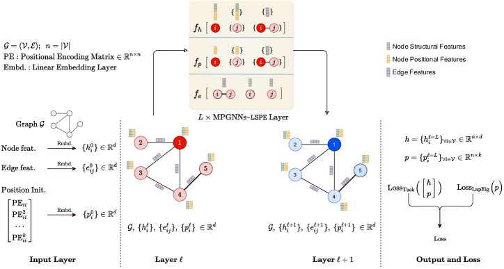
Typical usage: project the PE and add it to the projected node features, so the two live in the same space:
Computational Cost
Computing the \(k\) smallest non-trivial eigenvectors of an \(N \times N\) Laplacian:
- Dense (full eigendecomposition): \(O(N^3)\) time, \(O(N^2)\) memory, fine for a 30-atom molecule, infeasible beyond a few thousand nodes
- Sparse iterative (Lanczos / LOBPCG): each iteration costs \(O(k\lvert E\rvert)\), giving \(O(k\lvert E\rvert T)\) for \(T\) iterations
The iterative bound deserves a caveat: \(T\) is not a constant you control. It depends on the spectral gap separating the eigenvalues you want from the rest. On a graph with well-separated low eigenvalues convergence is fast; on one with a cluster of near-equal eigenvalues, exactly the degenerate case that also causes basis ambiguity, it can be slow, and the returned basis within the cluster is numerically unstable into the bargain. So the honest statement is that LapPE is cheap on small or well-separated graphs and unreliable in cost on large or highly symmetric ones. Random-walk PEs (next post) sidestep this entirely.
Worked Numerical Example
Consider the path graph \(P_4\): nodes \(1,2,3,4\) with edges \(1\)–\(2\), \(2\)–\(3\), \(3\)–\(4\).
The graph Laplacian is:
L = D - A =
[ 1  -1   0   0 ]
[-1   2  -1   0 ]
[ 0  -1   2  -1 ]
[ 0   0  -1   1 ]
For a path \(P_n\) the eigenvalues are \(\lambda_m = 2 - 2\cos\!\big(\pi (m-1)/n\big)\) and the eigenvectors are \(u_m(i) \propto \cos\!\big(\pi (m-1)(i - \tfrac12)/n\big)\). For \(n = 4\):
\(\lambda_1 = 0\), \(\lambda_2 = 2-\sqrt{2} \approx 0.586\), \(\lambda_3 = 2\), \(\lambda_4 = 2+\sqrt{2} \approx 3.414\).
Fiedler vector, normalised to unit length:
Node 1 sits at one extreme, node 4 at the other, and nodes 2 and 3 in between, recovering the linear order of the path. A GNN given these values as extra features can now separate node 1 from node 4 and node 2 from node 3, which no amount of message passing would achieve on its own.
But read the “or its negation” seriously. All four values flip together, and \(P_4\)’s reversal automorphism means node 1 and node 4 are automorphic: the encoding tells them apart only by sign, and a sign-invariant read-out puts them back together. What LapPE genuinely adds here is the relative geometry, that 1 and 4 are at opposite extremes while 2 and 3 are central.
What LapPE Can Distinguish
Adding any graph-derived feature to node inputs can only increase what an MPNN separates, so LapPE-augmented GNNs are at least as expressive as 1-WL, and there exist pairs they separate that 1-WL cannot, for example two nodes in a regular graph, where 1-WL assigns a single colour but the eigenvectors vary.
Three conditions temper that:
- Cospectral graphs. Two non-isomorphic graphs can share an identical Laplacian spectrum. Where the eigenvalues also fail to distinguish the relevant nodes, LapPE adds nothing that 1-WL did not already have.
- Automorphism. Nodes in the same automorphism orbit cannot be separated by any equivariant encoding.
- Invariance costs power. The sign- and basis-invariant treatments needed to make LapPE usable discard information. What you can actually exploit is what survives the invariantisation, not the raw eigenvector.
So: strictly more expressive than 1-WL on some inputs, not uniformly, and the gain depends on how the ambiguity is handled.
Summary
| Property | LapPE |
|---|---|
| Basis | Eigenvectors of the \(k\) smallest non-zero Laplacian eigenvalues |
| Captures | Low-frequency structure: community splits, coarse global geometry |
| Metric | Related to commute time, but the unweighted truncation is a proxy, not equal to it |
| Sign / basis issue | \(2^k\) sign choices, plus \(O(m)\) freedom in any multiplicity-\(m\) eigenspace |
| Cost | \(O(k\lvert E\rvert T)\) with a sparse solver, where \(T\) depends on the spectral gap |
| Expressiveness | Exceeds 1-WL on some pairs; automorphic nodes still tie |
| Used by | SAN, GPS, many Graph Transformer papers |
LapPE is the reference choice for graph positional encodings when low-frequency global position is what the task needs, the graph is small enough for a reliable eigensolve, and you are willing to handle sign and basis ambiguity properly.
References
- Belkin, M., & Niyogi, P. (2003). Laplacian Eigenmaps for Dimensionality Reduction and Data Representation. Neural Computation.
- Dwivedi, V. P., Lim, A. T., Beaini, D., & Lió, P. (2021). Graph Neural Networks with Learnable Structural and Positional Representations. ICLR 2022.
- Kreuzer, D., Beaini, D., Hamilton, W. L., Létourneau, V., & Tossou, P. (2021). Rethinking Graph Transformers with Spectral Attention. NeurIPS 2021 (SAN).