Graph Classification: From Node Embeddings to Graph Embeddings

The Graph Classification Pipeline

Given a dataset of graphs \(\{(G_1, y_1), \dots, (G_n, y_n)\}\), the goal is to learn a function \(f : G \mapsto y\). Unlike node classification (predict a per-node label) or link prediction (predict edge existence), graph classification must process entire graphs of varying sizes.

The standard pipeline:

Input graph G = (V, E, X)
         ↓
[Message Passing: K layers]
         ↓
Node embeddings {h^(K)_v : v ∈ V}
         ↓
[Readout: global pooling]
         ↓
Graph embedding h_G ∈ ℝ^d
         ↓
[MLP classifier]
         ↓
Prediction ŷ

Message Passing for Graph Classification

The message passing stage is the same as for node-level tasks. The only difference: we do not use the final node embeddings directly — we aggregate them.

JK-Net readout: rather than using only the last-layer embeddings, JK-Net concatenates each node’s intermediate embeddings across layers before pooling:

This is particularly useful for graph classification: different nodes may require different receptive field sizes, and keeping every layer’s output ensures no scale is lost to oversmoothing in the deepest layer.

Worked Example: Why Sum Beats Mean for Graph Classification

Consider two graphs both representing “benzene-like rings” but of different sizes:

• Graph A: 6 nodes, each with feature value 1. Mean pooling: 6/6 = 1.0. Sum pooling: 6.
• Graph B: 3 nodes, each with feature value 1. Mean pooling: 3/3 = 1.0. Sum pooling: 3.

Mean pooling gives identical embeddings for A and B — the classifier cannot distinguish them. Sum pooling gives 6 vs 3 — the size difference is captured. For tasks where ring size matters (e.g., predicting molecule toxicity), this distinction is critical.

The GIN Recipe for Graph Classification

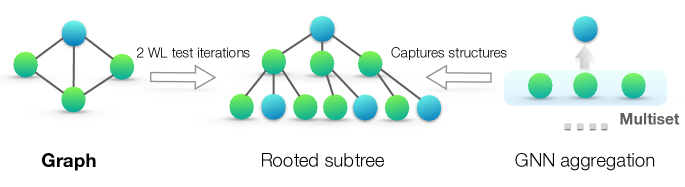
GIN (Graph Isomorphism Network) matches the 1-WL test — the strongest any message-passing GNN can be. For graph classification:

1. \(K\) layers of GIN message passing (sum aggregation + injective MLP)
2. Sum readout within each layer, concatenation across layers:

1. MLP classifier on \(h_G\) to produce \(\hat{y}\)

The combination of sum aggregation (injective over multisets), sum readout (preserves count information), and an MLP (universal approximator) reaches the maximum expressiveness available to an MPNN.

Benchmarks and Datasets

TUDatasets (standard graph classification benchmarks):

• MUTAG (188 graphs, 2 classes): mutagenic aromatic compounds
• PROTEINS (1113 graphs, 2 classes): enzyme vs non-enzyme proteins
• IMDB-B (1000 graphs, 2 classes): movie collaboration graphs
• REDDIT-B (2000 graphs, 2 classes): discussion thread graphs
• COLLAB (5000 graphs, 3 classes): collaboration networks

Note: these benchmarks have been criticised for high variance and potential data leakage. OGB (Open Graph Benchmark) provides more rigorous benchmarks.

OGB graph classification benchmarks:

• ogbg-molhiv: HIV activity prediction (41,127 molecules)
• ogbg-molpcba: molecular property prediction (437,929 molecules)
• ogbg-ppa: protein function prediction (158,100 protein interaction graphs)

What Actually Moves the Needle

Rather than quote accuracy figures — which on these datasets vary enormously with the split, the folds, and the hyperparameter budget — it is more useful to state the ordering that theory predicts and that ablations consistently reproduce:

• Swapping mean readout for sum is the single largest architectural change available on tasks whose label depends on counts or on graph size. It is a change in what the model can express, not a tuning improvement.
• Swapping GCN aggregation for GIN aggregation matters for the same reason one level down: it makes the neighbourhood aggregation injective rather than averaging.
• Hierarchical pooling (DiffPool, SAGPool) and learned readout (Set2Set, attention) help when the label depends on intermediate-scale structure that a single flat pool blurs away. When it does not, they mostly add parameters.

End-to-End Training Intuition

Intuition first. Think of graph classification like classifying handwritten digits: the convolutional layers (= message passing) extract local features; pooling (= readout) combines them into a fixed-size vector; the dense layers (= MLP) make the final call. The key difference is that graphs have no spatial grid — “pooling” must be permutation-invariant.

Common Failure Modes

Readout bottleneck: using mean pooling with a powerful GNN loses count information — two graphs with different sizes but proportionally identical node distributions get the same embedding.

Depth collapse: adding too many message passing layers → oversmoothing → all node embeddings identical → graph embeddings identical regardless of structure.

Benchmark overfitting: TUDataset benchmarks are small and high-variance. Performance differences < 2% should not be interpreted as meaningful without statistical testing.

End-to-End Training

The entire pipeline (GNN + readout + MLP) is trained end-to-end with a single loss (cross-entropy for classification, MSE for regression). The readout step admits gradients for all standard choices: sum, mean and max are differentiable almost everywhere; attention readout is smooth; DiffPool is fully differentiable through its soft assignment; TopKPool and SAGPool are differentiable only through the score gating — the top-\(k\) selection itself contributes no gradient, so dropped nodes receive no learning signal.

Summary

Graph classification ties together all the concepts in the pooling section: the choice of message passing determines per-node expressiveness; the readout determines what graph-level information is preserved; the MLP maps the graph summary to the prediction. Getting all three right is what separates random-chance performance from state-of-the-art.

References

• Xu, K., Hu, W., Leskovec, J., & Jegelka, S. (2019). How Powerful are Graph Neural Networks?. ICLR 2019 (GIN — most expressive MPNN for graph classification).
• Xu, K., Li, C., Tian, Y., Sonobe, T., Kawarabayashi, K., & Jegelka, S. (2018). Representation Learning on Graphs with Jumping Knowledge Networks. ICML 2018 (JK-Net readout).
• Hu, W., Fey, M., Zitnik, M., Dong, Y., Ren, H., Liu, B., Catasta, M., & Leskovec, J. (2020). Open Graph Benchmark: Datasets for Machine Learning on Graphs. NeurIPS 2020 (OGB benchmarks).